PDF-Calculation of the density of states in and dimensions We will here postulate that PDF document

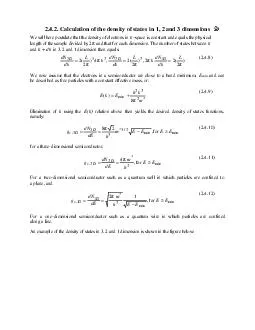
42 Calculation of the density of states in 1 2 and 3 dimensions We will here postulate that the density of electrons in space is constant and equals the physical

Upload by myesha-ticknor
Published on 2014-12-24

Presentation Embed Code

<iframe width="560" height="315" src="https://www.docslides.com/embed/28824" frameborder="0" allowfullscreen></iframe>

Download Presentation

Download Presentation The PPT/PDF document "Calculation of the density of states in ..." is the property of its rightful owner. Permission is granted to download and print the materials on this web site for personal, non-commercial use only, and to display it on your personal computer provided you do not modify the materials and that you retain all copyright notices contained in the materials. By downloading content from our website, you accept the terms of this agreement.