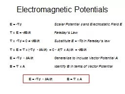
E f Scalar Potential f and Electrostatic Field E x E B t Faradays Law x f 0 B t ID: 618840
Download Presentation The PPT/PDF document "Electromagnetic Potentials" is the property of its rightful owner. Permission is granted to download and print the materials on this web site for personal, non-commercial use only, and to display it on your personal computer provided you do not modify the materials and that you retain all copyright notices contained in the materials. By downloading content from our website, you accept the terms of this agreement.
Slide1
Electromagnetic Potentials
E = -f Scalar Potential f and Electrostatic Field E x E = -∂B/∂t Faraday’s Law x -f = 0 ≠ -∂B/∂t Substitute E = -f in Faraday’s law x E = x (-f - ∂A/∂t) = 0 - ∂( x A)/∂t = -∂B/∂t E = -f - ∂A/∂t Generalize to include Vector Potential A B = x A Identify B in terms of Vector Potential E = -f - ∂A/∂t B = x ASlide2
Electromagnetic Potentials
(A,f) 4-vector generates E, B 3-vectors ((A,f) redundant by one degree) Suppose (A,f) and (A’,f’) generate the same E, B fields E = -f - ∂A/∂t = -f’ - ∂A’/∂t B = x A = x A’ Let A’ = A + f x A’ = x (A + f) = x A + x f = x A What change must be made to f to generate the same E field? E = -f’ - ∂A’/∂t = -f’ -
∂
(A + f )/∂t = -f - ∂A/∂t A’ = A + f f’ = f - ∂f/∂t Gauge Transformation Slide3
Electromagnetic Potentials
A = AL + AT L and T components of A A’ = AL + AT + f Change of gauge . A’ = . AL + . AT + . f = . AL + 2 f . AT = 0 Choose . A’ = 0 f = -AL A’ = AT f’ = f - ∂f/∂t f’ = f - ∂f/∂t f’ = f + ∂AL/∂t E = -f - ∂A/∂t = (-f
) -
∂(
AL+ AT)/∂t x E = x (-f - ∂A/∂t) = x -∂AT/∂t x f = x ∂AL/∂
t
= 0
E
= -
f
’
-
∂
A
’
/
∂
t =
(-
f
-
∂
A
L
/
∂
t) -
(∂
A
T
/
∂
t)
x
E
=
x -
∂
A
T
/
∂
tSlide4
Electromagnetic Potentials
Coulomb Gauge Choose . A = 0 Represent Maxwell laws in terms of A,f potentials and j, r sources x B = mo j + moeo ∂E/∂t Maxwell-Ampère Law x ( x A) = mo j + moeo ∂ (-f - ∂A/∂t)/∂t (. A) - A = mo j – 1/c2 ∂f/∂t - 1/c2 ∂ 2A/
∂
t
2
.
E = r /eo Gauss’ Law . (-f - ∂A/∂t) = -. f - ∂. A/∂t = - r /eo
Slide5
Electromagnetic Potentials
. A = 0 -2f = r /eo Coulomb or Transverse Gauge Coupled equations for A, fSlide6
Electromagnetic Potentials
Lorentz Gauge Choose . A = – 1/c2 ∂f/∂t x B = mo j + moeo ∂E/∂t Maxwell-Ampère Law (. A) - A = mo j – 1/c2 ∂f/∂t - 1/c2 ∂ 2A/∂t2 .
E
=
r /eo Gauss’ Law . (-f - ∂A/∂t) = -. f - ∂. A/∂t = -. f + 1/c2 ∂2f/∂t2 =
r
/
e
o
Slide7
Electromagnetic Potentials
. A = – 1/c2 ∂f/∂t Lorentz Gauge □2 □2 =
Slide8
Electromagnetic Potentials
□2 Each component of A, f obeys wave equation with a source □2 = □2G(r - r’, t - t’) = d(r - r’) d(t - t’) Defining relation for Green’s functiond(r - r’) d(t - t’) Represents a point source in space and time G(r - r’, t - t’) =
Proved by substitution
) is non-zero for
i.e. time taken for signal
to travel from
r
’ to
r
at speed c (retardation of the signal) ensures causality (no response if t’ > t) Slide9
Electromagnetic Potentials
Solution in terms of G and sourceLet
be the retardation time, then there is a contribution to
from
at t’ = t - . Hence we can write, more simply,
c.f.
GP
Eqn
13.11Similarly
c.f
.
GP
Eqn
13.12
These are
retarded vector and scalar potentials
Slide10
Radiation by Hertz Electric Dipole
+q-qlxyzr = (x, y, z) Field Pointr' = (0, 0, z’) Source PointCharge q(t) = qo Re {eiwt}Current I(t) = dq/dt = qo Re {iw eiwt}Dipole Moment p(t) = po Re {eiwt} = qo l Re {
e
i
wt} Wire Radius aCurrent Density j(t) = I(t) / p a2Using retarded potentials, calculate E(r,t), B(r
,t
) for dipole at originSlide11
Radiation by Hertz Electric Dipole
Retarded Electric Vector PotentialA(r, t) A || ez because j || ez Retardation time t = |r - ezz’| / c if l << c t then t ≈ |r| / c = r / cAz(r, t) for distances r >> l. A = – 1/c2 ∂f/∂t
Obtain
f
from Lorentz Gauge condition. A = ∂Az(r, t) / ∂z =
=
–
∂
f
/∂t
∂
f
/∂t =
Slide12
Radiation by Hertz Electric Dipole
Differentiate wrt z and integrate wrt t to obtainAz(r, t)
since d(t - r/c) =
dt
Charge q(t
) =
q
o
Re {
e
i
w
t
}
Current
I
(t
) =
=
q
o
Re {
i
w
eiwt
} Electric Field
E
(
r
, t) = -
f
-
Slide13
Radiation by Hertz Electric Dipole
Switch to spherical polar coordinates
-
k =
w
/ c
is the dipole amplitude
Slide14
Radiation by Hertz Electric Dipole
Obtain part of E field due to A vectorAz(r, t) Cartesian representationA(r, t) Spherical polar rep’n-
-
-
Slide15
R
adiation by Hertz Electric Dipole Total E fieldELong range (radiated) electric field, proportional to
E
rad
Radiated
E
field lines
,
polar plots
Slide16
Radiation by Hertz Electric Dipole
Short range, electrostatic field = 0 i.e. k = / c → 0Total E fieldE
E
electrostat
. = -
Classic field of electric point
dipole
Slide17
Radiation by Hertz Electric Dipole
Obtain B field from x A
A
(r,
t)
Radiated part of
B
field
t)
=
/ c
Slide18
Radiation by Hertz Electric Dipole
Power emitted by Hertz DipoleThe Poynting vector, N, gives the flux of radiated energy Jm-2s-1The flux N = E x H depends on r and q, but the angle-integrated flux is constantN = E x H = / mo
Slide19
Radiation by Hertz Electric Dipole
=
=
> =
Average
power over one cycle
Slide20
Radiation by Half-wave Antenna
l/2xyzr = (x, y, z) Field Pointr' = (0, 0, z’) Source Pointq’q
t –
t
–
I
(z’, t) =
I
o
cos
(2
p
z’/
l
)
e
i
w
t
Current distribution on wire is
half wavelength and harmonic in time
Half
W
ave
A
ntenna
r
r’
Current distributionSlide21
Radiation by Half-wave Antenna
Single Hertz Dipole = = / =
Current distribution in antenna
(z’, t) =
cos
Radiation from antenna is equivalent to sum of radiation from Hertz dipoles
t
–
t –
Slide22
Radiation by Half-wave Antenna
k =
Slide23
Radiation by Half-wave Antenna
Half Wave Antenna electric field
c.f.
GP 13.24 NB phase differenceHertz Dipole electric field
1
In general, for radiation in vacuum
B
=
k
x
E
/ c, hence for antenna
Slide24
Radiation by Half-wave Antenna
=
=
Average power over one cycle
Slide25
Radiation by Half-wave Antenna
Half Wave Antenna =
Polar plot for half wave antenna
Hertz Dipole
Polar
plot for
Hertz dipole
Slide26
Radiation by Half-wave Antenna
Full Wave Antenna
Hertz Dipole