/
9/10/10 A. Smith; based on slides by E. Demaine, C. Leiserson, S. Raskhodnikova, K. Wayne 9/10/10 A. Smith; based on slides by E. Demaine, C. Leiserson, S. Raskhodnikova, K. Wayne

9/10/10 A. Smith; based on slides by E. Demaine, C. Leiserson, S. Raskhodnikova, K. Wayne - PowerPoint Presentation

natalia-silvester
natalia-silvester . @natalia-silvester
Follow
342 views
Uploaded On 2019-06-21

9/10/10 A. Smith; based on slides by E. Demaine, C. Leiserson, S. Raskhodnikova, K. Wayne - PPT Presentation

Adam Smith Algorithm Design and Analysis L ECTURE 7 Greedy Graph Algorithms Topological sort Shortest paths CSE 565 The Algorithm Design Process Work out the answer for some examples Look for a general principle ID: 759609

Share:

Link:

Embed:

Download Presentation from below link

Download Presentation The PPT/PDF document "9/10/10 A. Smith; based on slides by E. ..." is the property of its rightful owner. Permission is granted to download and print the materials on this web site for personal, non-commercial use only, and to display it on your personal computer provided you do not modify the materials and that you retain all copyright notices contained in the materials. By downloading content from our website, you accept the terms of this agreement.


Presentation Transcript

Slide1

9/10/10

A. Smith; based on slides by E. Demaine, C. Leiserson, S. Raskhodnikova, K. Wayne

Adam Smith

Algorithm Design and Analysis

L

ECTURE 7Greedy Graph AlgorithmsTopological sortShortest paths

CSE

565

Slide2

The (Algorithm) Design Process

Work out the answer for some examplesLook for a general principleDoes it work on *all* your examples?Write pseudocodeTest your algorithm by hand or computerDoes it work on *all* your examples?Prove your algorithm is always correctCheck running timeBe prepared to go back to step 1!

9/10/10

A. Smith; based on slides by E. Demaine, C. Leiserson, S. Raskhodnikova, K. Wayne

Slide3

Writing algorithms

Clear and unambiguousTest: You should be able to hand it to any student in the class, and have them convert it into working code.Homework pitfalls:remember to specify data structureswriting recursive algorithms: don’t confuse the recursive subroutine with the first calllabel global variables clearly

9/10/10

A. Smith; based on slides by E. Demaine, C. Leiserson, S. Raskhodnikova, K. Wayne

Slide4

Writing proofs

PurposeDetermine for yourself that algorithm is correctConvince readerWho is your audience?YourselfYour classmateNot the TA/graderMain goal: Find your own mistakes

9/10/10

A. Smith; based on slides by E. Demaine, C. Leiserson, S. Raskhodnikova, K. Wayne

Slide5

Exploring a graph

Classic problem: Given vertices s,t ∈ V, is there a path from s to t?Idea: explore all vertices reachable from sTwo basic techniques:Breadth-first search (BFS)Explore children in order of distance to start nodeDepth-first search (DFS)Recursively explore vertex’s children before exploring siblings

9/10/10

A. Smith; based on slides by E. Demaine, C. Leiserson, S. Raskhodnikova, K. Wayne

How to convert these descriptions to precise algorithms?

Slide6

A. Smith; based on slides by E. Demaine, C. Leiserson, S. Raskhodnikova, K. Wayne

Adjacency-matrix representation

The adjacency matrix of a graph G = (V, E), where V = {1, 2, …, n}, is the matrix A[1 . . n, 1 . . n] given by

A

[i, j] =

1 if (i, j) ∈ E,0 if (i, j)  E.

2

1

3

4

A

1

2

3

4

1

2

3

4

0

1

1

0

0

0

1

0

0

0

0

0

0

0

1

0

Storage: ϴ(

V

2

)

Good for

dense

graphs.

Lookup:

O(1)

time

List all neighbors: O(|V|)

9/10/10

Slide7

Adjacency list representation

An adjacency list of a vertex v ∈ V is the list Adj[v] of vertices adjacent to v.

9/10/10

A. Smith; based on slides by E. Demaine, C. Leiserson, S. Raskhodnikova, K. Wayne

2

1

3

4

Adj

[1] = {2, 3}

Adj

[2] = {3}

Adj

[3] = {}Adj[4] = {3}

For undirected graphs, | Adj[v] | = degree(v).For digraphs, | Adj[v] | = out-degree(v).

How many entries in lists? 2|E| (“handshaking lemma”)Total ϴ(V + E) storage — good for sparse graphs.

Typical notation:

n

= |

V

|

= # vertices

m

= |

E

|

= # edges

Slide8

DFS pseudocode

Maintain a global counter timeMaintain for each vertex vTwo timestamps:v.d = time first discoveredv.f = time when finished“color”: v.color white = unexploredgray = in processblack = finishedParent v.π in DFS tree

9/10/10

A. Smith; based on slides by E. Demaine, C. Leiserson, S. Raskhodnikova, K. Wayne

Slide9

DFS pseudocode

Note: recursive function different from first call…Exercise: change code to set “parent” pointer?

9/10/10

A. Smith; based on slides by E. Demaine, C. Leiserson, S. Raskhodnikova, K. Wayne

Slide10

DFS example

T = tree edge (drawn in red)F = forward edge (to a descendant in DFS forest)B= back edge (to an ancestor in DFS forest)C = cross edge (goes to a vertex that is neither ancestor nor descendant)

9/10/10

A. Smith; based on slides by E. Demaine, C. Leiserson, S. Raskhodnikova, K. Wayne

Slide11

DFS with adjacency lists

Outer code runs once, takes time O(n) (not counting time to execute recursive calls)Recursive calls:Run once per vertextime = O(degree(v))Total: O(m+n)

9/10/10

A. Smith; based on slides by E. Demaine, C. Leiserson, S. Raskhodnikova, K. Wayne

Slide12

Toplogical Sort

9/10/10

A. Smith; based on slides by E. Demaine, C. Leiserson, S. Raskhodnikova, K. Wayne

Slide13

Directed Acyclic Graphs

Def. An DAG is a directed graph that contains no directed cycles.Ex. Precedence constraints: edge (vi, vj) means vi must precede vj.Def. A topological order of a directed graph G = (V, E) is an ordering of its nodes as v1, v2, …, vn so that for every edge (vi, vj) we have i < j.

a DAG

a topological ordering

v2

v3

v6

v5

v4

v7

v1

v

1

v

2

v

3

v

4

v

5

v

6

v

7

Slide14

Precedence Constraints

Precedence constraints. Edge (vi, vj) means task vi must occur before vj.Applications.Course prerequisite graph: course vi must be taken before vj.Compilation: module vi must be compiled before vj. Pipeline of computing jobs: output of job vi needed to determine input of job vj.Getting dressed

underwear

pants

jacket

shirt

boots

socks

mittens

Slide15

Recall from book

Every DAG has a topological orderIf G graph has a topological order, then G is a DAG.

9/10/10

A. Smith; based on slides by E. Demaine, C. Leiserson, S. Raskhodnikova, K. Wayne

Slide16

Review

Suppose your run DFS on a DAG G=(V,E)True or false?Sorting by discovery time gives a topological orderSorting by finish time gives a topological order

9/10/10

A. Smith; based on slides by E. Demaine, C. Leiserson, S. Raskhodnikova, K. Wayne

Slide17

Shortest Paths

9/10/10

A. Smith; based on slides by E. Demaine, C. Leiserson, S. Raskhodnikova, K. Wayne

Slide18

9/10/10

A. Smith; based on slides by E. Demaine, C. Leiserson, S. Raskhodnikova, K. Wayne

Shortest Path Problem

Input:Directed graph G = (V, E).Source node s, destination node t.for each edge e, length (e) = length of e.length path = sum of edge lengthsFind: shortest directed path from s to t.

Length of path (s,2,3,5,t)is 9 + 23 + 2 + 16 = 50.

s

3

t

2

6

7

4

5

23

18

2

9

14

15

5

30

20

44

16

11

6

19

6

Slide19

9/10/10

A. Smith; based on slides by E. Demaine, C. Leiserson, S. Raskhodnikova, K. Wayne

Rough algorithm (Dijkstra)

Maintain a set of explored nodes S whose shortest path distance d(u) from s to u is known.Initialize S = { s }, d(s) = 0.Repeatedly choose unexplored node v which minimizesadd v to S, and set d(v) = (v).

shortest path to some u in explored part, followed by a single edge (u, v)

s

v

u

d(u)

S

(e)

Slide20

9/10/10

A. Smith; based on slides by E. Demaine, C. Leiserson, S. Raskhodnikova, K. Wayne

Rough algorithm (

Dijkstra)

Maintain a set of explored nodes S whose shortest path distance d(u) from s to u is known.Initialize S = { s }, d(s) = 0.Repeatedly choose unexplored node v which minimizesadd v to S, and set d(v) = (v).

shortest path to some u in explored part, followed by a single edge (u, v)

s

v

u

d(u)

S

(e)

BFS with

weighted edges

Invariant:

d(u

) is known

for all vertices in S

Slide21

9/10/10

A. Smith; based on slides by E. Demaine, C. Leiserson, S. Raskhodnikova, K. Wayne

Demo of Dijkstra’s Algorithm

A

B

D

C

E

10

3

1

4

7

9

8

2

2

Graph with nonnegative edge lengths:

Slide22

9/10/10

A. Smith; based on slides by E. Demaine, C. Leiserson, S. Raskhodnikova, K. Wayne

Demo of Dijkstra’s Algorithm

A

B

D

C

E

10

3

1

4

7

9

8

2

2

Initialize:

A

B

C

D

E

Q:

0

¥

¥

¥

¥

S:

{}

0

¥

¥

¥

¥

Slide23

9/10/10

A. Smith; based on slides by E. Demaine, C. Leiserson, S. Raskhodnikova, K. Wayne

Demo of Dijkstra’s Algorithm

A

B

D

C

E

10

3

1

4

7

9

8

2

2

A

B

C

D

E

Q:

0

¥

¥

¥

¥

S:

{

A

}

0

¥

¥

¥

¥

“A”

E

XTRACT

-M

IN

(

Q

)

:

Slide24

9/10/10

A. Smith; based on slides by E. Demaine, C. Leiserson, S. Raskhodnikova, K. Wayne

Demo of Dijkstra’s Algorithm

A

B

D

C

E

10

3

1

4

7

9

8

2

2

A

B

C

D

E

Q:

0

¥

¥

¥

¥

S:

{

A

}

0

10

3

¥

¥

10

3

Explore edges leaving

A

:

¥

¥

Slide25

9/10/10

A. Smith; based on slides by E. Demaine, C. Leiserson, S. Raskhodnikova, K. Wayne

Demo of Dijkstra’s Algorithm

A

B

D

C

E

10

3

1

4

7

9

8

2

2

A

B

C

D

E

Q:

0

¥

¥

¥

¥

S:

{

A, C

}

0

10

3

¥

¥

10

3

“C”

E

XTRACT

-M

IN

(

Q

)

:

¥

¥

Slide26

9/10/10

A. Smith; based on slides by E. Demaine, C. Leiserson, S. Raskhodnikova, K. Wayne

Demo of Dijkstra’s Algorithm

A

B

D

C

E

10

3

1

4

7

9

8

2

2

A

B

C

D

E

Q:

0

¥

¥

¥

¥

S:

{

A, C

}

0

7

3

5

11

10

3

7

11

5

Explore edges leaving

C

:

¥

¥

Slide27

9/10/10

A. Smith; based on slides by E. Demaine, C. Leiserson, S. Raskhodnikova, K. Wayne

Demo of Dijkstra’s Algorithm

A

B

D

C

E

10

3

1

4

7

9

8

2

2

A

B

C

D

E

Q:

0

¥

¥

¥

¥

S:

{

A, C, E

}

0

7

3

5

11

10

3

7

11

5

“E”

E

XTRACT

-M

IN

(

Q

)

:

¥

¥

Slide28

9/10/10

A. Smith; based on slides by E. Demaine, C. Leiserson, S. Raskhodnikova, K. Wayne

Demo of Dijkstra’s Algorithm

A

B

D

C

E

10

3

1

4

7

9

8

2

2

A

B

C

D

E

Q:

0

¥

¥

¥

¥

S:

{

A, C, E

}

0

7

3

5

11

10

3

¥

¥

7

11

5

7

11

Explore edges leaving

E

:

Slide29

9/10/10

A. Smith; based on slides by E. Demaine, C. Leiserson, S. Raskhodnikova, K. Wayne

Demo of Dijkstra’s Algorithm

A

B

D

C

E

10

3

1

4

7

9

8

2

2

A

B

C

D

E

Q:

0

¥

¥

¥

¥

S:

{

A, C, E, B

}

0

7

3

5

11

10

3

¥

¥

7

11

5

7

11

“B”

E

XTRACT

-M

IN

(

Q

)

:

Slide30

9/10/10

A. Smith; based on slides by E. Demaine, C. Leiserson, S. Raskhodnikova, K. Wayne

Demo of Dijkstra’s Algorithm

A

B

D

C

E

10

3

1

4

7

9

8

2

2

A

B

C

D

E

Q:

0

¥

¥

¥

¥

S:

{

A, C, E, B

}

0

7

3

5

9

10

3

¥

¥

7

11

5

7

11

Explore edges leaving

B

:

9

Slide31

9/10/10

A. Smith; based on slides by E. Demaine, C. Leiserson, S. Raskhodnikova, K. Wayne

Demo of Dijkstra’s Algorithm

A

B

D

C

E

10

3

1

4

7

9

8

2

2

A

B

C

D

E

Q:

0

¥

¥

¥

¥

S:

{

A, C, E, B, D

}

0

7

3

5

9

10

3

¥

¥

7

11

5

7

11

9

“D”

E

XTRACT

-M

IN

(

Q

)

:

Slide32

9/10/10

A. Smith; based on slides by E. Demaine, C. Leiserson, S. Raskhodnikova, K. Wayne

Proof of Correctness (Greedy Stays Ahead)

Invariant. For each node u  S, d(u) is the length of the shortest path from s to u.Proof: (by induction on |S|)Base case: |S| = 1 is trivial.Inductive hypothesis: Assume for |S| = k  1.Let v be next node added to S, and let (u,v) be the chosen edge.The shortest s-u path plus (u,v) is an s-v path of length (v).Consider any s-v path P. We'll see that it's no shorter than (v).Let (x,y) be the first edge in P that leaves S,and let P' be the subpath to x.P + (x,y) has length · d(x)+ (x,y)· (y)· (v)

S

s

y

v

x

P

u

P'

Slide33

Review Question

Is Dijsktra’s algorithm correct with negative edge weights?

9/10/10

A. Smith; based on slides by E. Demaine, C. Leiserson, S. Raskhodnikova, K. Wayne

Slide34

9/10/10

A. Smith; based on slides by E. Demaine, C. Leiserson, S. Raskhodnikova, K. Wayne

Implementation

For unexplored nodes, maintainNext node to explore = node with minimum (v).When exploring v, for each edge e = (v,w), updateEfficient implementation: Maintain a priority queue of unexplored nodes, prioritized by (v).

Priority Queue

Slide35

Priority queues

Maintain a set of items with priorities (= “keys”)Example: jobs to be performedOperations:InsertIncrease keyDecrease keyExtract-min: find and remove item with least keyCommon data structure: heapTime: O(log n) per operation

9/10/10

A. Smith; based on slides by E. Demaine, C. Leiserson, S. Raskhodnikova, K. Wayne

Slide36

9/10/10

A. Smith; based on slides by E. Demaine, C. Leiserson, S. Raskhodnikova, K. Wayne

Pseudocode

for Dijkstra(G, )

d[s]  0for each v Î V – {s}do d[v]  ¥; p[v]  ¥S  Q  V ⊳ Q is a priority queue maintaining V – S, keyed on [v]

while Q ¹ do u  EXTRACT-MIN(Q)S  S È {u}; d[u]  p[u] for each v Î Adjacency-list[u]do if [v] > [u] + (u, v) then [v]  d[u] + (u, v)

explore edges leaving v

Implicit DECREASE-KEY

Slide37

9/10/10

A. Smith; based on slides by E. Demaine, C. Leiserson, S. Raskhodnikova, K. Wayne

Analysis of Dijkstra

degree

(

u)times

n

times

Handshaking Lemma

·

m implicit DECREASE-KEY’s.

while

Q ¹ do u  EXTRACT-MIN(Q)S  S È {u}for each v Î Adj[u]do if d[v] > d[u] + w(u, v) then d[v]  d[u] + w(u, v)

† Individual ops are amortized bounds

PQ Operation

ExtractMin

DecreaseKey

Binary heap

log n

log n

Fib heap †

log n

1

Array

n

1

Total

m log n

m + n log n

n2

Dijkstra

n

m

d-way Heap

HW3

HW3

m log

m/n

n