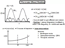
Phase Matching z I 2 k 2 gt k 1 Need k small to get efficient conversion Problem strong dispersion in refractive index with frequency in ID: 225287
Download Presentation The PPT/PDF document "Wavevector" is the property of its rightful owner. Permission is granted to download and print the materials on this web site for personal, non-commercial use only, and to display it on your personal computer provided you do not modify the materials and that you retain all copyright notices contained in the materials. By downloading content from our website, you accept the terms of this agreement.
Slide1
Wavevector (Phase) Matching
z
I
(2
)
k
2 > k1
Need k small to get efficient conversion- Problem – strong dispersion in refractive index with frequency in visible and near IR
n
= [n()-n(2)] 0 because of dispersion linear optics problem
n
(
)
2
Solutions:
Birefringent media
Quasi-phase-matching (QPM)
Waveguide solutionsSlide2
Birefringent Phase-Matching: Uniaxial Crystals
Uniaxial Crystals
0
0
0
0
0
0
=
0
“ordinary” refractive
index “
extraordinary” refractive index
- optically isotropic in the
x
-
y
plane
-
z
-axis is the “optic axis”
- for , any two orthogonal directions
are equivalent
eigenmode
axes
cannot phase-match for
x
y
z
x
y
z
in
x
-
z
plane
in
x
-
z
plane,
n
e
(
)
along
y
-axis,
n
o
Convention
:
- Note: all orthogonal axes in
x
-
y
plane
are equivalent for linear optics
always in
x
-
y
plane
always
has
z
component
- angle from
x
-axis important for Slide3
Type I Phase-Match
1 fundamental
eigenmode
1 harmonic
eigenmode
+
ve uniaxial
ne>no
no(2) =
ne(,)+ve uniaxial oee
Fundamental (need 2 identical photons)
Harmonic (1 photon)
k
= 2ke
(
) – ko
(2) = 2kvac
()
[n
e(
,
)-no
(2
]
E
n
e
n
o
Non-critical
phase-match
=
/2
n
o
(2
) =
n
e
(
)
x
y
z
e
E
o
E
x
y
z
e
E
o
Critical
phase-match 0<
<
/2
n
o
(2
)
=
n
e
(
,
)
n
e
(
,
)
n
o
n
e
n
(
)
n
(
)Slide4
Because of optical isotropy in
x
-
y
plane
for phase-matching lies on a cone
at an angle
from the z-axis lies in x-y plane
Note:
does
depend on angle
from x-axis in x-y plane!!
Range
of phase-match frequencies limited
by condition
n
e()
no(2
)Slide5
Type I -ve uniaxial
no>n
e
-
ve
uniaxial
eoono(
) = ne(,2)Harmonic
Fundamental
k = 2ko() – ke(2
) = 2k
vac(
)[no
()-ne
(,2
]
Critical
phase-match 0<
</2
n
e
(
)
n
o
n
e
n
(
)
Non-critical
phase-match
=/2
n
o
n
e
n
(
)Slide6
Type II Phase-Match
2 fundamental
eigenmodes
1 harmonic
eigenmode
+
ve
uniaxial oeo
Fundamentals, need 2 (orthogonally polarized) photons
Harmonic (1 photon)
k
= ke() + ko() – ko
(2
) =
kv
ac(){
[ne(,
)+
no
()] - 2
no(2
)}
n
e
n
o
n
(
)
+
ve
uniaxial
n
e
>
n
o
Slide7
-ve
uniaxial
e
oe
Harmonic
Fundamental
k
=
k
e
() + ko() – ke(2
)= k
vac(
)[n
e(,
) + no()] -
kvac
(2)
ne
(,2
) = k
v
ac
(
){
[
n
e
(
,
)
+
n
o
(
)] - 2
n
e
(
,2)}
Unique
n
(
)
ne
n
o
Type II -
ve uniaxial
no
>
ne Slide8
n
e
(2
,
)
n
o(2
)ne(,)
n
o
()
Z
(optic) axis
PM
Poynting
vectors
“Critical” Phase Match
“Non-Critical” Phase Match
n
o
(
)
=
n
e
(2
)
Curves are tangent
Difference between the
normals
to
the curves represent spatial walk-off
between fundamental and harmonic
Reduces
conversion efficiency
Type I
eooSlide9
“Critical” Versus “Non-Critical” Phase Match
How precise must
PM
be? I
(2
) sinc2[
kL/2= /2] 4/2 0.5
0
e.g. Type I eoo
(-ve uniaxial
)
Usually quote the “full”
acceptance angle = 2
PM
PM
(Half width at half
maximum)
I(2
,
)
Note key role of birefringenceSlide10
Non-collinear Phase-MatchingWe have discussed only collinear
wavevector
matching. However, clearly it is possible to
extend the wavelength range of
birefringent phase-matching
by tilting the beams.
Biggest disadvantage: Walk-off
Interaction limited to this region
Small birefringence is an advantage in maintaining a useful angular bandwidthSlide11
Quasi-Phase-Matching
k
= 2
k
e
(
) – ke
(2) + pK
- direction of is periodically reversed along a ferroelectric crystalPeriodically poled LiNbO3(PPLN):
x
z
p
’th
Fourier component
Change phase-matching condition
by
manufacturing different
1
a
>0
a
is the “mark-space
ratio”
PPLNSlide12
A – perfect phase match with
B – QPM with p=1
C -
Quasi-Phase-Matching: Properties (1)
c/
n
(2
)
n
(
)
x
A modified form of
“non-critical” phase-match
zSlide13
The relative strengths of the Fourier components
depend
on
a
.
k
= 2
k
e() – ke(2) + pK
Not
useful since
Not useful because
Phase matching is possible
Higher order gratings can be used to extend phase-matching to
shorter wavelengths, although the nonlinearity does drop
off,
Quasi-Phase-Matching: Properties (2)Slide14
fundamental and harmonic co-polarized
d
(2)
eff
16 pm/V
(p
=1) samples up to 8
cms long conversion efficiency 1000%/W (waveguides) commercially available from many sources still some damage issues
Right-hand side picture shows blue,green-yellow and red beams obtained by doubling 0.82, 1.06 and 1.3 mcompact lasers in QPM LiNbO3State-of-the-art QPM LiNbO3 Slide15
Solutions to Type 1 SHG Coupled Wave Equations
-first assume
negligible fundamental depletion valid to
10% conversion
E(2
) and
E() are /2 out of phase at
L=0!!!e.g. Type I
2
E(
)
E(
)
E(2
)
Large Conversion Efficiency
(assume energy is conserved
Kleinman
limit)
Field NormalizationSlide16
Normalized Coupling Constant
Normalized
Propagation
Distance
Normalized
Wavevector
Detuning
“Global Phase”
Inserting into coupled wave equations and separating into real and imaginary equations
I
ntegrated by
the method of the variation of the
parameters Slide17
Sgn
is
determined by the
sign of
boundary (initial) condition sine(
)
The general solution is given in terms of Jacobi elliptic function
Solutions simplify for
s
=0
,
i.e. on phase-matchThe conversion efficiency saturates at unity (as expected
)Slide18
Δs=0.2
Δ
s0
(
solid black line);
(dashed
black line);
(
red dashed line); (solid blue line, curve multiplied by factor of 4).
The main
(
Δ
k=0) peak with increasinginput which means that the tuning bandwidthbecomes progressively narrower.
The side-lobes become progressively
narrowerand their peaks shift to smaller
ΔkL.
Δs=0.2
z
I
(2
)
k
2
>
k
1
Note the different shape of the harmonic
response compared to low depletion caseSlide19
Solutions to Type 2 SHG Coupled Wave Equations
2
E
3
(2
)
E
1
(
)
E
2
(
)
Normalizations
Physically useful solutions are given in terms of the photon fluxes
N
(
)
, i.e. photons/unit area
Simple analytical solutions can only be given for the case
Δ
s
=0
Slide20
No asymptotic final state
All intensities are periodic
with distance
Oscillation period depends
on input intensities
Type 2 SHG: Phase-Matched