/
Word Sense Discrimination Word Sense Discrimination

Word Sense Discrimination - PDF document

natalia-silvester
natalia-silvester . @natalia-silvester
Follow
383 views
Uploaded On 2015-10-19

Word Sense Discrimination - PPT Presentation

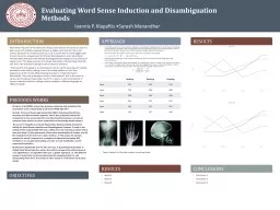
Schitze Xerox Palo Alto Research Center paper presents contextgroup discrimination a disambiguation algorithm based on cluster ing Senses are interpreted as groups or clusters of similar cont ID: 165812

Sch{itze* Xerox Palo Alto Research

Share:

Link:

Embed:

Download Presentation from below link

Download Pdf The PPT/PDF document "Word Sense Discrimination" is the property of its rightful owner. Permission is granted to download and print the materials on this web site for personal, non-commercial use only, and to display it on your personal computer provided you do not modify the materials and that you retain all copyright notices contained in the materials. By downloading content from our website, you accept the terms of this agreement.


Presentation Transcript

Word Sense Discrimination Sch{itze* Xerox Palo Alto Research Center paper presents context-group discrimination, a disambiguation algorithm based on cluster- ing. Senses are interpreted as groups (or clusters) of similar contexts of the ambiguous word. Words, contexts, and senses are represented in Word Space, a high-dimensional, real-valued space in which closeness corresponds to semantic 1. Introduction sense disambiguation is the task of assigning sense labels to occurrences of an ambiguous word. This problem can be divided into two subproblems: sense discrimi- nation and sense labeling. Sense discrimination divides the * Xerox Palo Alto Research Center, 3333 Coyote Hill Road, Palo Alto, CA 94304 Q 1998 Association for Computational Linguistics Linguistics Volume 24, Number 1 We therefore call our approach sense discrimination, since we do not require manually constructed sources of knowledge. In many applications, word sense disambiguation must both discriminate and la- bel occurrences; for example, in order to find the correct translation of an ambiguous word in machine translation or the right pronunciation in a text-to-speech system. The application of interest to us is information access, i.e., making sense of and find- ing information in large text databases. For many problems in information access, it is sufficient to solve the discrimination problem only. In one study, we measured document-query similarity based on word senses rather than words and achieved a considerable improvement in ranking relevant documents ahead of nonrelevant doc- uments (Schi.itze and Pedersen 1995). Since the measurement of similarity is a system- internal process, no reference to externally defined senses need be made. Another potentially beneficial application of word sense discrimination in information access is the design of interfaces that take account of ambiguity. If a user enters a query that contains an ambiguous word, a system capable of discrimination can give examples of the different senses of the word in the text database. The user can then decide which sense was intended and only documents with the intended sense would be retrieved. Again, a reference to external sense definitions is not required for this task. The algorithm we propose in this paper is context-group discrimination. 1 Context- group discrimination groups the occurrences of an ambiguous word into clusters, where clusters consist of contextually similar occurrences. Words, contexts, and clus- ters are represented in a high-dimensional, real-valued vector space. Context vectors capture the information present in second-order co-occurrence. Instead of forming a context representation from the words that the ambiguous word directly occurs with in a particular context (first-order co-occurrence), we form the context represen- tation from the words that these words in turn co-occur with in the training corpus. Second-order co-occurrence information is less sparse and more robust than first-order information. In context-group discrimination, the context of each occurrence of the ambiguous word in the training corpus is represented as a context vector formed from second- order co-occurrence information. The context vectors are then clustered into coherent groups such that occurrences judged similar according to second-order co-occurrence are assigned to the same cluster. Clusters are represented by their centroids, the av- erage of their elements. An occurrence in a test text is disambiguated by computing the second-order representation of the relevant context, and assigning it to the cluster whose centroid is closest to that representation. Since the choice of representation influ- ences the formation of clusters, we will experiment with several representations in this paper, some involving a dimensionality reduction using singular value decomposition (SVD). Context-group discrimination can be generalized to do a discrimination task that goes beyond the notion of sense that underlies many other contributions to the dis- ambiguation literature. If the ambiguous word's occurrences are clustered into a large number n of clusters (e.g., n = 10), then the clusters can capture fine contextual distinc- tions. Consider the example of a small number of clusters, only the senses "outer space" and "limited extent in one, two, or three dimensions" are separated. If the word's occurrences are clustered into more clusters, then finer distinctions such as the one between "office space" and "exhibition space" are also discovered. Note that differences between sense entries in dictionaries are often similarly fine-grained. The basic idea of the algorithm was first described in Schi~tze (1992b). Automatic Word Sense Discrimination WORD I TRAINING TEXT VECTORS I WORD SPACE ----T:xxOx! ~x xi/ Xx~." '......x. ", CONTEXT / 1 basic design of context-group discrimination. Contexts of the ambiguous word in the training set are mapped to context vectors in Word Space (upper dashed arrow) by summing the vectors of the words in the context. The context vectors are grouped into clusters (dotted lines) and represented by sense vectors, their centroids (squares). A context of the ambiguous word ("test context") is disambiguated by mapping a context vector in Word Space (lower dashed arrow ending in circle). The context is assigned to the sense with the closest sense vector (solid arrow). Even if the contextual distinctions captured by generalized context-group discrimina- tion do not line up perfectly with finer distinctions made in dictionaries, they still help characterize the contextual meaning in which the ambiguous word is used in a partic- ular instance. Such a characterization is useful for the information-access applications described above, among others. The basic idea of context-group discrimination is to induce senses from contextual similarity. There is some evidence that contextual similarity also plays a crucial role in human semantic categorization. Miller and Charles (1991) found evidence in several experiments that humans determine the semantic similarity of words from the similar- ity of the contexts they are used in. We hypothesize that, by extension, senses are also based on contextual similarity: a sense is a group of contextually similar occurrences of a word. The following sections describe the disambiguation algorithm, our evaluation, and the results of the algorithm for a test set drawn from the York Times Wire, and discuss the relevance of our approach in the context of other work on word sense disambiguation. Context-Group Discrimination discrimination groups a set of contextually similar occurrences of an ambiguous word into a cluster, which is then interpreted as a sense. The particular im- plementation of this idea described here makes use of a high-dimensional, real-valued vector space. Context-group discrimination is a corpus-based method: all representa- tions are derived from a large text corpus. The basic design of context-group discrimination is shown in Figure 1. Each oc- currence of the ambiguous word in the training set is mapped to a point in Word Space (shown for one example occurrence: see dashed line from training text to Word Space). The mapping is based on word vectors that are looked up in Word Space (to be described below). Once all training-text contexts have been mapped to Word Space, the resulting point cloud is clustered into groups of points such that points are close to each other in each group and that groups are as distant from each other as 99 Linguistics Volume 24, Number 1 possible. The resulting clusters are delimited by dotted lines in the figure. Each cluster is assumed to correspond to a sense of the ambiguous word (an assumption to be evaluated later). The representative of each group is its centroid, depicted as a square. After training, a new occurrence of the ambiguous word (labeled "test context" in the figure) is disambiguated by mapping its context to Word Space (see lower dashed line; the context's point is depicted as a circle). The context is then assigned to the context group whose centroid is closest (solid arrow). Finally, the context is categorized as being a use of the sense corresponding to this context group. There are three types of entities that we need to represent: words, contexts, and senses. They are represented as word vectors, context vectors, and sense vectors, re- spectively. Word vectors are derived from neighbors in the corpus, context vectors are derived from word vectors, and sense vectors are derived by way of clustering from the distribution of context vectors. The representational medium of a vector space was chosen because of its wide acceptance in information retrieval (IR) (see, e.g., Salton and McGill 1983). The vector- space model is arguably the most common framework in IR. Systems based on it have ranked among the best in many evaluations of IR performance (Harman 1993). The success of the vector-space model motivates us to use it for the representation of words. We represent words in a space in which each dimension corresponds to a word, just as documents and queries are commonly represented in this space in IR. Another approach to computing word similarity is the representation of words in a document space in which each dimension corresponds to a document (Lesk 1969; Salton 1971; Qiu and Frei 1993). There are fewer occurrence-in-document than word- co-occurrence events, so these word representations tend to be more sparse and, ar- guably, less informative than word-based representations. Word vectors have also been based on hand-encoded features (Gallant 1991) and dictionaries (Sparck-Jones 1986; Wilks et al. 1990). Corpus-based methods like the one proposed here have the ad- vantage that no manual labor is required and that a possible mismatch between a general dictionary and a specialized text (e.g., on chemistry) is avoided. Finally, word similarity can be computed from structural features like head-modifier relationships (Grefenstette 1994b; Ruge 1992; Dagan, Marcus, and Markovitch 1993; Pereira, Tishby, and Lee 1993; Dagan, Pereira, and Lee 1994). Like document-based representations, structure-based representations are sparser than those based on co-occurrence. It is debatable whether structural features are more informative than associational features (Grefenstette 1992, 1996) or not (Schtitze and Pedersen 1997). Approaches to word representation closely related to ours were proposed by Niwa and Nitta (1994) and Burgess and Lund (1997). Instead of co-occurrence counts, vector entries are mutual information scores between the word that is to be represented and the dimension words, in Niwa and Nitta's approach. The algorithms for vector derivation and sense discrimination are described in what follows. 2.1 Word Vectors A vector for word w is derived from the close neighbors of w in the corpus. Close neighbors are all words that co-occur with w in a sentence or a larger context. In the simplest case, the vector has an entry for each word that occurs in the corpus. The entry for word v in the vector for w records the number of times that word v occurs close to w in the corpus. It is this representational vector space that we refer to as WOrd Space. Figure 2 gives a schematic example of two words being represented in a two- dimensional space. The representation is based on the co-occurrence counts of a hypo- 100 Automatic Word Sense Discrimination Table 1 Co-occurrence counts for four words in a hypothetical corpus. The words interpreted as dimensions in Figure 2, vectors. Vector Dimension robe legal 133 200 300 JUDGE f f/ ROBE I I 75 200 CLOTHES 2 The derivation of word vectors, represented as word vectors in a two-dimensional space with the dimensions 'legal' and 'clothes.' Co-occurrence data are from Table 1. thetical corpus in Table 1. The word a value of 300 on the dimension "legal" because 300 times with each other (see below for which words are selected as dimensions; a word can be a dimension of Word Space and represented as a word vector in Word Space at the same time). This vector representation captures the typical topic or subject matter of a word. For example, words like closer to the "legal" dimension; words like closer to the "clothes" dimension. By looking at the amount of overlap between two vectors, one can roughly determine how closely they are related semantically. This is because related meanings are often expressed by similar sets of words. Semantically related words will therefore co-occur with similar neighbors and their vectors will have considerable overlap. This similarity can be measured by the cosine between two vectors. The cosine is equivalent to the normalized correlation coefficient: fi, ~ ) ~iN=l ViWi ff and ~ are vectors and N is the dimension of the vector space. The value of the cosine is higher, the more overlap there is between the neighbors of the two words whose vectors are compared. If two words occur with exactly the same neighbors 101 Linguistics Volume 24, Number 1 (perfect overlap), then the value of the cosine is 1.0. If there is no overlap at all, then the value of the cosine is 0.0. The cosine can therefore be used as a rough measure of semantic relatedness between words. What words should serve as the dimensions of Word Space? We will experiment with two strategies: a global and a local one. The local strategy focuses on the contexts of the ambiguous words and ignores the rest of the corpus. The global strategy is to select the n most frequent words of the corpus as features and use them regardless of the word that is to be disambiguated. (See Karov and Edelman 1996 for a different approach that selects features according to a combination of global frequency and local salience.) For local selection, we can also use a frequency cutoff. As an alternative, we will test selection according to a X 2 test. For the frequency-based selection criterion, the neighbors of the ambiguous word in the corpus are counted. A neighbor is any word that occurs at a distance of at most 25 words from the ambiguous word (that is, in a 50- word window centered on the ambiguous word). The 1,000 most frequent neighbors are chosen as the dimensions of the space. For the x2-based criterion, a x2-measure of dependence is applied to a contingency table containing the number of contexts of the ambiguous word in which the candidate word occurs (N++) and does not occur (N+_), and the number of contexts without an occurrence of the ambiguous word in which the candidate word occurs (N_+) and does not occur (N__). = N(N++N__ - 2 + N+_)(N_+ + N__)(N++ + N_+)(N+_ + N__) underlying assumption in using the x2-test is that candidate words whose occur- rence depends on whether the ambiguous word occurs will be indicative of one of the senses of the ambiguous word and hence useful for disambiguation. 2 After 1,000 words have been selected in local selection, word vectors are formed by collecting a 1,000-by-I, 000 matrix C, such that element the number of times that words i and j co-occur in a window of size k. Column n (or, equivalently, row n) of matrix C represents word n. Note that C is symmetric since the words that are represented as word vectors are also those that form the dimensions of the 1,000- dimensional space. We chose a window size of k = 50 because no improvement of discrimination performance was found in Schfitze (1997) for k � 50. For global selection, we choose the 20,000 most frequent words as features and the 2,000 most frequent words as dimensions of Word Space. A global 20, 000-by-2, 000 co-occurrence matrix is derived from the corpus. Association data were extracted from the training set consisting of 17 months of the York Times Service, June 1989 through October 1990. The size of this set is about 435 megabytes and 60.5 million words. Two months (November 1990 and May 1989; 46 megabytes, 5.4 million words) were set aside as a test set. Context Vectors representation for words derived above conflates senses. For example, both senses of the word and 'garment') are summed in its word vector, which will therefore be positioned somewhere between the 'legal' and 'clothes' dimensions in Figure 2. We need to go back to individual contexts in the corpus to acquire information about sense distinctions. Contexts are represented as context vectors in Word Space. Candidate words are selected after a list of 930 stopwords has been removed. This stop list was based on the one used in the Text Data Base system (Cutting, Pedersen, and Halvorsen 1991). Automatic Word Sense Discrimination CENTROID / ~JUDGE / I I /// 3 The derivation of context vectors. A context vector is computed as the centroid of the words occurring in the context. The words in this example context are law, judge, statute, and suit. A context vector is the centroid (or sum) of the vectors of the words occurring in the context. Figure 3 shows the context vector of an example context of suit containing the words law, judge, statute, and suit. Note that the context vector is closer to the "legal' than to the 'clothes' dimension, thus capturing that the context is a 'legal' use of suit. (The true sum of the four vectors is longer than shown. Since all correlation coefficients are normalized, the length of a vector does not play a role in the computations.) The centroid "averages" the direction of a set of vectors. If many of the words in a context have a strong component for one of the topics (like 'legal' in Figure 3), then the average of the vectors, the context vector, will also have a strong component for the topic. Conversely, if only one or two words represent a particular topic, then the context vector will be weak on this component. The context vector hence represents the strength of different topical or semantic components in a context. In the computation of the context vector, we will weight a word vector according to its discriminating potential. A rough measure of how well word wi discriminates between different topics is the log inverse document frequency used in information retrieval (Salton and Buckley 1990): ai = l°g/~ / where ni is the number of documents that wi occurs in and N is the total number of documents. Poor discriminators of topics are words such as idea or help that are relatively uniformly distributed and therefore have a high document frequency. Good content discriminators like automobile or China have a bursty distribution (they have several occurrences in a short interval if they occur at all Church and Gale 1995), and therefore a low document frequency relative to their absolute frequency. Other algorithms for computing context vectors have been proposed by Wilks et al. (1990) (based on dictionary entries), Gallant (1991) (based on hand-encoded semantic features), Grefenstette (1994b) (based on light parsing), and Niwa and Nitta (1994) (a comparison of dictionary-based and corpus-based context vectors). 103 Linguistics Volume 24, Number 1 1 Cl ..,,,7 ,s ~- SENSE 4 The derivation of sense vectors. Sense vectors are derived by clustering the context vectors of an ambiguous word (here, cl, c2, c3, c4, c5, c6, c7, and computing sense vectors as the centroids of the resulting clusters. The vectors SENSE 1 and SENSE 2 are the sense vectors of clusters {cl, c2, c3, c4} and {cs, c6, c7, 2.3 Sense Vectors Sense representations are computed as groups of similar contexts. All contexts of the ambiguous word are collected from the corpus. For each context, a context vector is computed. This set of context vectors is then clustered into a predetermined number of coherent clusters or context groups using Buckshot (Cutting et al. 1992), a combination of the EM algorithm and agglomerative clustering. The representation of a sense is simply the centroid of its cluster. It marks the portion of the multidimensional space that is occupied by the cluster. We chose the EM algorithm for clustering since it is guaranteed to converge on a locally optimal solution of the clustering problem. In our case, the solution is optimal in that the sum of the squared distances between context vectors and their centroids will be minimal. In other words, the centroids are optimal representatives for the context vectors in their cluster. One problem with the EM algorithm is that it finds a solution that is only locally optimal. It is therefore important to find a good starting point since a bad starting point will lead to a local minimum that is not globally optimal. Some experimental evidence given below shows that cluster quality varies considerably depending on the initial parameters. In order to find a good starting point, we use group-average agglomerative clustering (GAAC) on a sample of context vectors. For each of the 2,000 clustering experiments described below, we first choose a random sample of 50. This size is roughly equal to v'~, the number of context vectors to be clustered. Since GAAC is of time complexity O(n2), this guarantees overall linear time complexity of the clustering procedure. If the training set has more than 2,000 instances of the ambiguous word, 2,000 context vectors are selected randomly. The centroids of the resulting clusters are then the parameters for the first iteration of EM. We compute five iterations of the EM algorithm for all experiments since in most cases only a few, if any, context vectors were reassigned in the fifth iteration. Both the EM algorithm and group-average agglomerative clustering are described in more detail in the appendix. 104 Automatic Word Sense Discrimination An example is shown in Figure 4. The clustering step has grouped context vectors cl, c2, c3, and c4 in the first group and c5, c6, c7, and c8 in the second group. The sense vector of the first group is the centroid labeled SENSE 1, the sense vector of the second group the centroid labeled SENSE 2. The result of clustering depends on the representation of context vectors. For this reason, we also investigate a transformation of the multidimensional space via a singular value decomposition (SVD) (Golub and van Loan 1989). SVD is a form of dimensionality reduction that finds the major axes of variation in Word Space. Context vectors can then be represented by their values on these principal dimensions. The motivation for applying SVD here is much the same as the use of Latent Semantic Indexing (LSI) in information retrieval (Deerwester et al. 1990). LSI abstracts away from the surface word-based representation and detects underlying features. When similarity is computed on these features (via cosine between SVD-reduced context vectors), contextual similarity can be, potentially, better measured than via cosine be- tween unreduced context vectors. The appendix defines SVD and gives an example matrix decomposition. In this paper, the word vectors will be reduced to 100 dimensions. The experiments reported in Schfitze (1992b, 1997) give evidence that reduction to this dimensionality does not decrease accuracy of sense discrimination. Space requirements for context vectors are reduced to about 1/10 and 1/20 for a 1,000-dimensional and a 2,000- dimensional Word Space, respectively. Although most word vectors are sparse, context vectors are dense, since they are the sum of many word vectors. Time efficiency is increased on the same order of magnitude when the correlation of context vectors and sense vectors is computed. The computation of the SVD's in this paper took from a few minutes per word for the local feature set to about three hours for the global feature set. Application of Context-Group Discrimination discrimination uses word vectors and sense vectors as follows to dis- criminate occurrences of the ambiguous word. For an occurrence t of the ambiguous word v: • Map t into its corresponding context vector ~ in Word Space using the vectors of the words in t's context (the lower dashed line in Figure 1). • Retrieve all sense vectors ~j of v (the two points marked as squares in the figure). • Assign t to the sense j whose sense vector ~j is closest to ~ (assignment shown as a solid arrow). This algorithm selects the context group whose sense vector is closest to the context vector of the occurrence of the word that is to be disambiguated. Context vectors and sense vectors capture semantic characteristics of the corresponding context and sense, respectively. Consequently, the sense vector that is closest to the context vector has the best semantic match with the context. Therefore, context-group discrimination categorizes the occurrence as belonging to that sense. Evaluation test context-group discrimination on the 10 natural ambiguous words that formed the test set in Schfitze (1992b) and on 10 artificial ambiguous words. Table 2 glosses the major senses of the 20 words. 105 Linguistics Volume 24, Number 1 2 of occurrences of test words in training and test set, percent rare senses in test set, baseline performance (all occurrences assigned to most frequent sense), and the two main senses of each of the 20 artificial and natural ambiguous words used in the experiment. Word Training Test. Rare Senses Baseline Frequent Senses range/ consulting firm 149 0% 62% disease/ reserve board 115 0% 54% development/ cease fire 101 0% 50% administration / fernando valley 122 0% wide range consulting firm heart disease reserve board urban development cease fire 52% drug administration fernando valley development / right field 88 0% 68% park/ judiciary committee 122 0% 70% companies / city hall 208 0% 58% dealers / paine webber 104 0% 55% baseball/ square feet 143 0% 66% rose/ nuclear power 103 0% 52% 200 2% 64% 200 4% 58% 200 0% 55% 200 0% 54% economic development right field national park judiciary committee japanese companies city hall drug dealers paine webber league baseball square feet pete rose nuclear power stock of goods seat of government a feeling of special attention a charge for borrowed money movement proposal for action a factory living being 106 Automatic Word Sense Discrimination 2 Word Training Test Rare Senses Baseline Frequent Senses 200 3.5% 60% an authoritative decision to exert control, or influence 200 0% 56% area, volume outer space 200 12.5% 57% an action or process in a court a set of garments 200 4.5% 90% a combat vehicle a receptacle for liquids 200 1.5% 74% a line of railroad cars to teach 144 13.9% 69% a ship or plane a tube or canal (as an artery) Artificial ambiguous words or pseudowords are a convenient means of testing disambiguation algorithms (Schtitze 1992a; Gale, Church, and Yarowsky 1992). It is time-consuming to hand-label a large number of instances of an ambiguous word for evaluating the performance of a disambiguation algorithm. Pseudowords circumvent this need: Two or more words, e.g., conflated into a new type: occurrences of either word in the corpus are then replaced by the new type. It is easy to evaluate disambiguation performance for pseudowords since one can go back to the original text to decide whether a correct decision was made. To create the pseudowords shown in Table 2, all word pairs were extracted from the corpus, i.e., all pairs of words that occurred adjacent to each other in the corpus in a particular order. All numbers were discarded, since numbers do not seem to involve sense ambiguity. Pseudowords were then created by randomly drawing two pairs from those that had a frequency between 500 and 1,000 in the corpus. Pseudowords were generated from pairs rather than simple words because pairs are less likely than words to be ambiguous themselves. Pair-based pseudowords are therefore good examples of ambiguous words with two clearly distinct senses. Table 2 indicates how often the ambiguous word occurred in the training and test sets, how many instances were instances of rare senses, and the baseline performance that is achieved by assigning all occurrences to the most frequent sense. In the eval- uation given here, only senses that account for at least 15% of the occurrences of the ambiguous word are taken into account. Rare senses are those that account for fewer than 15% of the occurrences. The words in Table 2 each had two frequent senses. The frequency of rare senses ranges from 0% to 13.9%, with an average of 2.1%. Rare senses are not eliminated from the training set. The training and test sets were taken from the York Times Service as described above (training set: June 1989-October 1990; test set: November 1990, May 1989). If a word had more than 200 occurrences in the test set, then only the first 200 occurrences were included in the evaluation. The labeling of words in the test corpus was performed by the author. The distinc- 107 Linguistics Volume 24, Number 1 tions between the senses in Table 2 are intuitively clear. For example, the probability of a context in which at the same time refer to a set of garments and an action in court is very low. Consequently, there were fewer than five instances where the appropriate sense was not obvious from the immediate context. In these cases, the sense that seemed more plausible to the author was assigned. It is important to evaluate on a test set that is separate from the training set. Context-group discrimination is based on the distribution of context vectors in the training set. The distribution in the training set is often a bad model for the distribution in the test set. In practice, the intended text of application will be from a time period not covered in the training set (for example, newswire text from after the date of training). Word distributions can change considerably over time. The test set was therefore constructed to be from a time period different from the time period of the training set. This is also the reason that we do not do cross-validation. Cross-validation respecting the constraint that test and training sets be from different time periods would have required a test set several times larger than the one that was available. Clustering and evaluating on the same set is also problematic because of sampling variation. Consider the following example. We have a set of three context vectors C {C 1 : c2 = (2), 3 : in a one-dimensional space. Contexts 1 and 2 are uses of sense 1, context 3 is a use of sense 2. If C is used as both training and evaluation set, then average performance is 83% (with probability 0.5, we get centroids 1.5 and 3 and 100% accuracy, with probability 0.5, we get centroids 1 and 2.5 and 67% accuracy). If we split C into a training set T of size 2 and a test set E of size 1, we get an average performance of 67% (100% for E = {cl}, 50% for E = {c2}, 50% for E {£3}), is lower than 83%. This example shows that conflating training and test set can result in artificially high performance. An advantage of context-group discrimination is that the granularity of sense distinctions is an adjustable parameter of the algorithm. Experiments run directly for the senses in Table 2 will test the algorithm's ability to discriminate coarse sense distinctions. To test performance for fine-grained sense distinctions (e.g., 'office space' vs. 'exhibition space'), we will run two experiments, one that evaluates performance for clustering the context vectors of a word into ten clusters and an information retrieval experiment in which the number of clusters is also large for sufficiently frequent words. The goal of the 10-cluster experiments is to induce more fine-grained sense distinc- tions than in the 2-cluster experiments. However, it is harder to determine the ground truth for fine sense distinctions. When it comes to fine distinctions, a large number of occurrences are indeterminate or compatible with several of the more finely individ- uated senses (cf. Kilgarriff 1993). For this reason, experiments with a large number of clusters were evaluated using two indirect measures. The first measure is accuracy for two-way discriminations, i.e., the degree to which each of the ten clusters contained only one of the two "coarse" senses. This evaluation is indirect because a cluster that contains, say, only 'limited extent in one, two, or three dimensions' uses of be deemed 100% correct, yet it could be randomly mixed as far as fine sense distinctions are concerned (e.g., 'office space' vs. 'exhibition space'). The author inspected the data and found good separation of fine-grained senses in the 10-cluster experiments to the extent that the evaluation measure indicated good performance on the two-way discrimination task. However, because of the above-mentioned subjectivity of judgements for fine sense distinctions, this is hard to quantify. Results from a second evaluation on an information retrieval task will be presented in Section 4.2 below. We will show that sense-based information retrieval (in which the relevance of documents to a query is determined using context-group discrimination) 108 Automatic Word Sense Discrimination improves the performance of an IR system considerably. Since the success of sense- based retrieval depends on the accuracy of context-group discrimination, we can infer that the algorithm reliably assigns ambiguous instances to induced senses even in the fine-grained case. 4. Experiments 4.1 Word Sense Discrimination Table 3 shows experimental results for context-group discrimination. There were four conditions that were varied in the experiments (as described in Section 2): • local vs. global feature selection • feature selection according to frequency 2 • term representations vs. SVD-reduced representations • number of clusters (2 vs. 10) For local feature selection, the other three parameters are varied systematically (the first eight columns of Table 3). For global feature selection, selection according to X 2 is not possible, since the X 2 test presupposes an event (like the occurrence of an ambiguous word) that the occurrence of candidate words depends on. There is no such event for global feature selection. A larger number of dimensions (2,000) is used for the global variant of the algorithm in order to get coverage of a large range of topics that might be relevant for disambiguation. We therefore apply SVD in the global feature selection case. Even if word vectors are sparse, context vectors are usually not. Clustering 2,000- dimensional vectors is computationally expensive, so that we only ran experiments with SVD-reduced vectors for the global variant. Ten experiments with different randomly chosen initial parameters were run for each of the 200 combinations of the different levels of Word, Representation, and Clustering. The mean percentage correctness and the standard deviation for each such set of 10 experiments is shown in the cells of Table 3. We give mean and deviation of the percentage of correctly labeled occurrences of all instances in the training set ("total" = "t.'), of the instances of sense 1 ("$1") and of the instances of sense 2 ("$2"). The bottom row of the table gives averages of the total percentage correct numbers over the 20 words covered. The rightmost column gives averages of the means over the 10 experiments. We analyzed the results in Table 3 via analysis of variance (ANOVA, see, for example, Ott 1992). An ANOVA was performed for a 20 x 5 x 2 design with 10 replicates. The factors were Word, Representation (local, frequency-based, terms; local, frequency-based, SVD; local, Xa-based, terms; local, x2-based, SVD; global, frequency- based, SVD), and Clustering (coarse = 2 clusters, fine = 10 clusters). Percentages were transformed using the functionf(X) = 2 x sin -1 (v/X) as recommended by Winer (1971). The transformed percentages have a distribution that is close to a normal distribution as required for the application of ANOVA. We found that the effects of all three factors and all interactions was significant at the 0.001 level. These effects are discussed in what follows. Word. general, performance for pseudowords is better than for natural words. This can be explained by the fact that pseudowords have two focussed senses--the two word pairs they are composed of. In contrast, some of the senses of natural ambiguous 109 Linguistics Volume 24, Number 1 Table 3 Results of disambiguation experiments. Rows give total accuracy for each word ("t.') as well as accuracy for the two senses separately ("$1", "$2"). The average in the bottom row is an average over total ("t.') accuracy numbers only. Columns describe experimental conditions and the mean ("~") and standard deviation ("a") of 10 replications of each experiment. The rightmost column contains an average over the mean values of the 10 experiments. Pseudowords are abbreviated to the first words of pairs. Global wide~consul. $2 55 16 100 0 69 31 92 9 74 25 92 13 69 24 82 10 89 6 94 4 t. 51 4 62 0 60 4 66 3 56 6 64 3 65 8 66 2 87 3 87 3 66 0 78 11 100 0 99 4. 72 0 75 12 100 0 98 2 100 0 100 0 $2 100 0 90 7 100 0 100 0 100 0 94 5 98 0 100 1 100 0 100 0 84 0:85 100 0 99 287 0 85 3 99 0 99 1 100 0 100 0 86 1 87 2 96 0 97 191 4 90 8 98 0 98 1 100 0 98 2 .ocon./right nat./jud. iap./city X 2 Frequency Frequency Terms SVD Terms I SVD SVD 2 10 2 10 2 10 2 10 2 10 45 16 0 0 45 47 22 22 25 26 19 30 59 37 39 17 84 2 76 8 41.4 81.6 66.4 88.8 98.2 93.8 94.1 $2 78 l J 70 7 100 0 100 1 73 24 80 11 100 0 96 5 100 0 100 0 89.7 t. 82 0i 79 3 98 0 99 1 I 82 10 85 3 99 0 97 2 100 0 99 1 92.0 S1 89 l i 87 7 98 0 100 1 I 94 4 88 5 98 0 95 1 100 0 100 0 94.9 $2 78 1 77 12 95 0 100 1 60 35 90 7 59 8 96 2 100 0 100 1 85.5 t. 84 I 82 3 97 0 100 0 78 15 89 2 80 4 96 1 100 0 100 0 90.6 $1 72 2 89 6 92 1 95 1 92 0 87 5 98 0 98 3 100 0 100 0 92.3 $2 89 0 67 13 96 0 96 2 87 2 91 5 96 0 97 2 100 0 100 0 91.9 t. 78 1 82 1 93 1 95 1 90 1 88 2 98 0 97 1 100 0 100 0 92.1 S1 91 1 96 3 98 0 97 0 99 0 99 0 98 01 97 1 100 0 100 0 97.5 $2 73 0 53 14 100 0 100 1 70 0 61 9 92 0i 96 4 100 0 98 2 84.3 t. 85 1 83 3 98 0 98 0 90 0 87 3 96 0i 97 1 100 0 99 1 93.3 84 18 90 7 96 1 95 1 94 2 91 4 97 2 93 2 99 0 99 1 93.8 56 10 63 15 71 23 87 4 66 17 71 10 88 5 90 5 99 0 99 1 79.0 t. 73 12 79 3 86 9 92 1 82 6 83 2 93 1 92 1 99 0 99 0 87.8 68 6 76 9 86 1 81 9 70 18 81 14 95 0 85 4 100 0 97 3 83.9 $2 86 13 86 8 100 0 99 1 68 23 87 14 100 0 98 3 100 0 100 0 92.4 t. 76 9 80 2 93 0 89 5 69 19 83 3 97 0 91 2 100 0 98 2 87.6 54 8 77 8 66 41 96 3 32 31 77 10 56 32 90 4 100 0 100 1 74.-----8 $2 60 20 94 3 100 0 99 1 91 18 94 5 100 0 96 4 100 0 99 2 93.3 t. 58 16 88 1 88 14 98 2 71 13 88 1 85 11 94 3 100 0 99 li 86.9 91 0 78 10 94 1 98 2 72 21 90 10 86 19 95 6 100 0 99 1 90.3 $2 78 0 80 8 94 0 91 2 96 1 81 13 88 20 91 7 100 0 99 1 I 89.8 t. 84 0 79 2 94 0 95 2 83 11 86 3 87 19 93 4 100 0 99 1 90.0 88 16 97 3 91 4 96 2 91 3 97 3 93 1 93 2 92 1 93 1 93.1 $2 27 23 36 11 23 34 87 7 36 34 57 9 80 27 88 6 96 1 89 5 61.9 t. 66 7 75 3 66 13 93 2 71 13 82 2 88 10 91 1 94 0 91 1; 81.7 82 18 77 8 95 1 86 5 96 0 93 3 94 1 91 4 96 0 89 3 89.9 $2 43 37 87 4 90 6 96 2 83 1 85 3 71 35 91 4 88 1 93 31 82.7 t. 66 14 81 4 93 2 90 2 90 0 90 1 84 15 91 2 93 0 91 li 86.9 57 14 72 6 58 1 84 1 61 17 88 6 90 15 93 4 85 1 91 5 I 77.-----------9 $2 60 15 70 10 97 0 91 8 58 20 63 16 51 24 77 7 88 13 71 151 72.6 t. 58 10 71 3 76 1 87 3 59 12 77 4 73 12 86 2 86 5 82 5 i 75.5 20 0 0 92 4 " 0 0 91 16 0 0 54 46 2 5 70 37 0 0' 38.-----2 $2 47 12 100 0 37 5 100 0 41 30 100 0 59 36 100 0 70 26 100 0 75.4 t. 59 8 54 0 63 4 54 0 64 11 54 0 56 7 55 2 70 13 54 0 58.3 75 1 61 13 84 2 71 14 81 1 65 15 79 7 79 13 85 0 82 3 76.2 $2 86 1 90 4 93 1 96 3 87 1 93 4 93 5 95 2 95 0 95 1 92.3 t. 82 0 78 3 90 1 86 4 84 0 82 4 88 1 89 4 91 0 90 1 86.0 10 25 48 30 0 0 48 22 15 25 38 24 16 25 51 15 8 25 54 16 28.8 $2 87 7 91 7 96 0 95 3 97 1 96 2 96 2 96 2 94 10 93 3 94.1 t. 53 7 72 9 54 0 74 8 61 11 71 10 60 12 76 6 56 5 75 6 65.2 83 1 77 5 80 2 85 6 81 2 84 7 94 2 88 8 95 0 83 6 85.0 $2 80 0 i 84 4 93 0 94 2 92 2 88 6 86 29 97 2 96 0 97 2 90.7 t. 82 1 I 80 2 85 1 89 3 86 1 86 2 91 12 92 4 95 0 89 3 87.5 29 91 7 6 80 8 32 13 88 5 12 14 86 29i~ 31 22 92 3 28 19 48.5 $2 94 15 100 0 92 95 1 100 0 87 5 99 2 84 1 99 2 94.9 4 99 0 t. 87 13 I 90 1 90 3 92 1 95 1 91 1 87 2i 92 1 85 1 92 2 90.1 60 21 100 0 74 16 100 0 89 20 100 0 95 81100 1 79 19 100 0 89.7 $2 40 21 0 0 12 20 0 0 18 29 0 0 8 21! 1 3 55 31 0 0 13.4 t. 55 10' 74 0 58 7 74 0 69 11 74 0 72 1' 74 0 73 8 74 0 69.7 84 18 86 14 100 0 99 1 85 30 90 7 20 42 94 2 30 48 79 5 76.7 $2 76 14 84 9 100 0 100 0 89 3 92 5 79 17 100 0 81 9 100 0 90.1 t. 79 15 85 2 100 0 100 0 88 11 91 2 61 14 98 1 65 13 93 1 .. 86.O i 72.1 I 77.9 84.1 i 88.5 i 77.8 i 81.8 i 82.9 88.3 i 89.7 i 90.6 I Automatic Word Sense Discrimination 4 Tukey W test shows significantly different performance for the five representations. Proportions are transformed using = 2 x sin -1 The rightmost column contains the accuracy A in percent that would correspond to the average value Y in the second column (i.e., = Y). difference for a = 0.01:0.034 Average of Difference Corresponding Level 2 x Closest Accuracy local, )/2, terms 2.11 0.13 76% local, frequency, terms 2.24 0.13 81% local, frequency, SVD 2.44 0.06 88% local, X 2, SVD 2.50 0.06 90% global, frequency, SVD 2.66 0.16 94% words (for example, composed of many different subsenses that are hard to identify for both people and computers. The only pseudoword with poor performance is range/consultingfirm. is an illustrative example of a weakness of the particular implementation of context- group discrimination chosen here. Since we only rely on topical information, a word composed of a nontopical sense, like range, can occur in almost any subject area is disambiguated poorly. The 'area, volume' sense of the 'teaching' sense of similarly topically amorphous and therefore hard if only topical informa- tion is considered. The poor performance for 'plant' in the 10-cluster experiments is probably due to the way training-set clusters were assigned to senses. The training set was clustered into 20 clusters and each cluster was given a sense label. This proce- dure introduces many misclassifications of individual instances in the training set. In contrast, a performance of 92% was achieved in Schiitze (1992b) by hand-categorizing the training set, instance by instance. Note that for some experimental conditions and for some words, performance of two-group clustering is below baseline. In a completely unsupervised setting, we have to make the assumption that the two induced clusters correspond to two different senses. In the worst case, we will get, two clusters with identical proportions of the two senses and an accuracy of 50%, below the baseline of assigning all occurrences to a sense that occurs in more than 50% of all cases. For example, for worst case would be two clusters each with 69% 'ship' instances and 31% 'tube' instances. Overall accuracy would be 0.5 x .69 + 0.5 x .31 = 0.5. It could be argued that the true baseline for unsupervised two-group clustering is 50%, not the proportion of the most frequent sense. Representation. Tukey W test (Ott 1992) was performed to evaluate the factor Representation. The Tukey W test determines the least significant difference between sample means. That is, it yields a threshold such that if two levels of a factor differ by more than the threshold, then they are significantly different. For the factor Rep- resentation, in our case, this least significant difference is 0.034 for a = 0.01. Table 4 shows that all differences are significant. This is evidence that SVD representations perform better than term representations and that global representations perform bet- ter than local representations. The advantage of SVD representations is partly due to the use of a normality assumption in clustering. This is a poor approximation for term 111 Linguistics Volume 24, Number 1 5 of selected term features in the test set. The table shows number of words occurring in the test set (averaged over the 20 ambiguous words); number of words occurring per context (averaged over contexts); proportion of words from one representation occurring in another (averaged first over contexts, then over ambiguous words; e.g., on average 91% of X2-selected terms were also in the set selected by local frequency); average number of contexts that a selected term occurred in (e.g., on average a xa-selected term occurred in 8.7 contexts of the artificial ambiguous words, averaged over the words in a context). Frequency Global Frequency Words Occurring in Test Set 283.0 571.2 489.6 Words per Context 6.1 11.1 9.2 Term Overlap 2 91% 53% local frequency 51% 100% 68% global frequency 34% 78% 100% Average Frequency of terms artificial words 8.7 6.7 16.7 natural words 39.5 22.4 17.5 representations, but is more accurate for SVD-reduced representations. Why do globally selected features perform better? Table 5 presents data on the occurrence of selected terms in the test set that are relevant to this question. Note first that locally selected features seem to do better than globally selected ones on several measures. More locally selected features occur in the test set ("words occurring in test set": 571.2 vs. 489.6), more local features occur in the individual contexts ("words per context": 11.1 vs. 9.2), and more global features are also local features than vice versa (on a per-context basis, 78% of global features are also local features, but only 68% of local features are also global features), suggesting that local features capture more information than global features. The first two measures also show that X2-selected features suffer from sparseness. Both the total number of features that occur in the training set and the number of words per context are small. This evidence explains why SVD representations that address sparseness do better than term representations for X 2. To explain the difference in performance between local and global frequency fea- tures, we have to break down average accuracy according to artificial and natural ambiguous words. Average accuracy for artificial ambiguous words is 89.9% (2 clus- ters) and 92.2% (10 clusters) for local features and 98.6% (2 clusters) and 98.0% (10 clusters) for global features. Average accuracy for natural ambiguous words is 76.0% (2 clusters) and 84.4% (10 clusters) for local features and 80.8% (2 clusters) and 83.1% (10 clusters) for global features. These data show a clear split. Performance of local and global features is comparable for natural ambiguous words. Global features perform clearly better for artificial ambiguous words. The last two rows of Table 5 explain this difference in behavior. The numbers corre- spond to the average number of contexts that the selected features occur in (averaged first over the words in a context, then over contexts; e.g., a context with three selected terms occurring in 10, 3, and 15 contexts of the ambiguous word in the training set would have an average number of contexts of (10+3+15)/3 = 9.3). These averages are 11.2 Automatic Word Sense Discrimination small for 2 local frequency in the case of artificial ambiguous words. Clustering can only work well if contexts have enough elements in common so that similarity can be determined robustly. Apparently, there were too few elements in common for X 2 and local frequency in the case of artificial ambiguous word (and the patterns were so sparse that even SVD was not an effective remedy). The problem is that artificial ambiguous words are much less frequent in the training set than natural ambiguous words (average frequencies of 1,306.9 vs. 8,231.0), so that reliable feature selection is harder for artificial ambiguous words. With ample information on natural ambiguous words available in the training set, features can be selected that will occur densely in the test set. The quality of feature selection for artificial ambiguous words was less successful due to smaller training set sizes. This analysis reiterates the importance of a clear separation of training and test sets. Performance numbers will be artificially high if feature selection is done on both training and test sets, avoiding the problems with feature coverage demonstrated in Table 5. Since global feature selection is simpler and as effective as local approaches, global feature selection is the preferred implementation of context-group discrimination in the general case. Note, however, that different words may have different optimal repre- sentations. For example, local features work best for are similar individual differences for frequency vs. x2-based selection. Frequency-based selection is best for x2-based selection is better for least for SVD-reduced representations. Clustering. clustering is generally better than coarse clustering. The one case for which coarse clustering comes close to the performance of fine clustering is global feature selection. But this small difference is almost entirely due to the bad performance of fine clustering for is likely to be due to insufficient hand- categorization of the training set, as explained above. That fine clustering performs better than coarse clustering is not surprising, since more information is used in the evaluation of fine clustering: the labeling of clus- ters in the training set. Only coarse clustering is evaluated as strictly unsupervised disambiguation, since we do not have an evaluation set for fine sense distinctions. general, the variance of discrimination accuracy is higher for coarse clus- tering than for fine clustering. This is not surprising, given the fact that we evaluate both types of clustering on how well they do on a two-way distinction. There may be several quite different ways of dividing a set of context vectors into two groups. But if we first cluster into ten groups and assign these groups to two senses, then the resulting two-way partitions are more likely to resemble each other (even if the initial 10-group clusterings are not very similar). The experiments indicate that context-group discrimination based on globally se- lected features is the best implementation in the general case. The algorithm achieves above-baseline performance (with a small number of exceptions for certain parameter settings). The average performance of the SVD-based representations of 83% to 91% is satisfactory, although inferior by about 5% to 10%, to disambiguation with minimal manual intervention (e.g., Yarowsky 1995). 3 3 Manually supplied priming information about senses is not the only difference between context-group discrimination and other disambiguation algorithms. Could one of the other differences be responsible for the difference in performance? The fact that the error rate more than doubles when the seeds in Yarowsky's (1995) experiments are reduced from a sense's best collocations to just one word per sense suggests that the error rate would increase further if no seeds were provided. 113 Linguistics Volume 24, Number 1 Application to Information Retrieval principal motivation for concentrating on the discrimination subtask is to ap- ply disambiguation to information retrieval. While there is evidence that ambiguity resolution improves the performance of IR systems (Krovetz and Croft 1992), several researchers have failed to achieve consistent experimental improvements for practi- cally realistic rates of disambiguation accuracy. Voorhees (1993) compared two term-expansion methods for information retrieval queries, one in which each term was expanded with all related terms and one in which it was only expanded with terms related to the sense used in the query. She found that disambiguation did not improve the performance of term expansion. In our study, we will use disambiguation to eliminate document-query matches that are due to sense mismatches (that is, the word in question is used in different types of context in the query and the document). This approach decreases the number of documents that a query matches with whereas term expansion increases it. Another important difference in this study is that longer queries are used. Long queries (as they may arise in an IR system after relevance feedback) provide more context than the short queries Voorhees worked with in her experiments. Sanderson (1994) modified a test collection by creating pseudowords similar to the ones used in this study. He found that even unrealistically high rates of disambiguation accuracy had little or no effect on retrieval performance. An analysis presented in Schfitze and Pedersen (1995) suggests that the main reason for the minor effect of disambiguation is that most of the pseudowords created in the study had a major sense that accounted for almost all occurrences of the pseudoword. Creating this type of pseudoword amounts to adding a small amount of noise to an unambiguous word, which is not expbcted to have a large effect on retrieval performance. To some extent, actual dictionary senses have the same property: one sense often accounts for a large proportion of occurrences. However, this is not necessarily true when rare senses are not taken into account and when high-frequency senses are broken up into smaller groups (the example of 'office space' vs. 'exhibition space'). Large dictionaries tend to break up high-frequency senses into such more narrowly defined subsenses. The successful use of disambiguation in our study may be due to the fact that rare senses, which are less likely to be useful in IR, are not taken into account and that frequent senses are further subdivided. Good evidence for the potential utility of disambiguation in information retrieval was provided by Krovetz and Croft (1992). They showed that there is a considerable amount of ambiguity even in technical text (which is often assumed to be less ambigu- ous than nonspecialized writing). Many technical terms have nontechnical meanings that are used in addition to more specialized senses even in technical text (e.g., computer magazines, automobile magazines Krovetz 1997). Krovetz and Croft also showed that sense mismatches (i.e., spurious matching words that were used in different senses in query and document) occurred significantly more often in nonrelevant than in relevant documents. This suggests that eliminating spurious matches could improve the separation between nonrelevant and relevant documents and hence the overall quality of retrieval results. In order to show that context-group discrimination is an approach to disambigua- tion that is beneficial in information retrieval, we will now summarize the experiment presented in Schfitze and Pedersen (1995). That experiment evaluates sense-based re- trieval, a modification of the standard vector-space model in information retrieval. (We refer to the standard vector-space model as word-based retrieval.) In word-based re- trieval, documents and queries are represented as vectors in a multidimensional space in which each dimension corresponds to a word (similar to the way that we repre- Automatic Word Sense Discrimination sent word vectors in Word Space). In sense-based retrieval, documents and queries are also represented in a multidimensional space, but its dimensions are words. Words are disambiguated using context-group discrimination. Documents and queries that contain a word assigned to a particular sense have a nonzero value on the corresponding dimension. The test corpus in Sch~tze and Pedersen (1995) is the Category B TREC-1 collection (about 170,000 documents from the Street Journal) conjunction with its queries 51-75 (Harman 1993). Sense-based retrieval improved average precision by 7.4% when compared to word-based retrieval. A combination of word-based and sense-based retrieval increased performance by 14.4%. The greater improvement of the combination is probably due to discrimination errors (i.e., the fact that discrimination is less than 100% correct), which are partially undone by combining sense and word evidence. Improvement was particularly high when small sets of documents were requested, for example, 16.5% (sense-based) and 19.4% (word- and sense-based combined) for a recall level of 10% of relevant documents. This experiment suggests a high utility of sense discrimination for information retrieval. At first sight, sense-based retrieval may seem related to term expansion. Both sense-based retrieval and term expansion take individual terms as the starting point for modifying the similarity measure that determines which documents are deemed most closely related to the query. However, the two approaches are actually opposites of each other in the following sense. Term expansion number of match- ing documents for a query. For example, if the query contains expan- sion adds documents containing additional nonzero matches. Sense-based retrieval number of matches. For example, if the word in the query and is disambiguated as being used in the 'legal' sense, then documents that contain a different sense will no longer match with the query. Discussion distinguishes context-group discrimination from other work on disambiguation is that no outside source of information need be supplied as input to the algorithm. Other disambiguation algorithms employ various sources of information. Kelly and Stone (1975) consider hand-constructed disambiguation rules; Lesk (1986), Krovetz and Croft (1989), Guthrie et al. (1991), and Karov and Edelman (1996) use on-line dic- tionaries; Hirst (1987) constructs knowledge bases; Cottrell (1989) uses syntactic and semantic structure encoded in a connectionist net; Brown et al. (1991) and Church and Gale (1991) exploit bilingual corpora; Dagan, Itai, and Schwall (1991) use a bilingual dictionary; Hearst (1991), Leacock, Towell, and Voorhees (1993), Niwa and Nitta (1994), and Bruce and Wiebe (1994) exploit a hand-labeled training set; and Yarowsky (1992) and Walker and Amsler (1986) perform computations based on a hand-constructed semantic categorization of words Thesaurus Longman's subject codes, re- spectively). For some of these algorithms, the expense of supplying information to the disam- biguation algorithm is relatively small. For example, in many of the methods using hand-labeled training sets (e.g., Hearst 1991), a relatively small number of training examples is sufficient. Yarowsky has proposed an algorithm that requires as little user input as one seed word per sense to start the training process (Yarowsky 1995). Such minimal user input will be a negligible burden for users in some situations. However, consider the interactive information-access application described above. When asked to improve their initial ambiguous information request many users will be reluctant to 115 Linguistics Volume 24, Number 1 give a seed word or a set of good features for each sense of the word. They are more likely to satisfy a request by the system to choose the correct sense (e.g., by mouse click), if example contexts corresponding to different senses are presented without the requirement of additional user interaction. In an application like this, it is of great ad- vantage that context-group discrimination does not require any manual intervention to induce senses. Another body of related work is the literature on word clustering in computational linguistics (Brown et al. 1992; Finch 1993; Pereira, Tishby, and Lee 1993; Grefenstette 1994a) and document clustering in information retrieval (van Rijsbergen 1979; Willett 1988; Sparck-Jones 1991; Cutting et al. 1992). In contrast to this earlier work, we cluster contexts or, equivalently, word tokens here, not words (or, more precisely, word types) or documents. The straightforward extension of word-type clustering and document clustering to word-token clustering would be to represent a token by all words it co- occurs with in its context and cluster these representations. Such an approach based on first-order co-occurrence is used, for example, by Hearst and Plaunt (1993) for the representation of tiles or document subunits that are similar to our notion of context. Instead, we use second-order co-occurrence to represent the tokens of ambiguous words: the words that occur with the token are in turn looked up in the training corpus and the words they co-occur with are used to represent the token. Second- order representations are less sparse and more robust than first-order representations. In a cluster-based approach, the subdivision of the universe of elements into clus- ters depends on the representation. If the representation does not capture the infor- mation crucial for distinguishing senses, then context-group discrimination performs poorly. The clearest such example in the above experiments is the pseudoword wide range~consulting firm. The algorithm does not do better than the baseline of always choosing the most frequent sense. The reason is that the representation captures only topic information. So a cluster will contain a group of contexts that are about the same topic. Unfortunately, the pair wide range can come up in text about almost any topic. Since there is no clear topical characterization of one sense of the pseudoword, context-group discrimination performs poorly. The reliance on topical similarity may also be the reason that performance for pseudowords is generally better than performance for natural ambiguous words. All pseudowords except for wide range/consultingJirm are composed of two pairs from dif- ferent topics. For example, heart disease and reserve board pertain to biology and finance, respectively, two clearly distinct topics. On the other hand, the senses of some of the ambiguous words have less clear associations with particular topics. For example, one can be trained to perform a wide variety of activities, so the 'teaching' sense of train can be invoked in many different topics. Part of the superior performance for pseu- dowords is due to this different topic sensitivity of natural and artificial ambiguous words. The limitation to topical distinctions is not so much a flaw of context-group dis- crimination as a flaw of the particular implementation we have presented here. It is possible to integrate information in the context vectors that reflect syntactic or sub- categorization behavior of different senses, such as the output of a shallow parser as used in Pereira, Tishby, and Lee (1993). For example, one good indicator of the two senses of the word interest is a preposition occurring to its right. The phrase interest in invokes the 'feeling of attention' sense, the phrase interest on, the sense 'charge on borrowed money.' It seems plausible that performance could be improved for words whose senses are less sensitive to topical distinctions if such "proximity" information is integrated. In some recent experiments, Pedersen and Bruce (1997) have used proxim- ity features (tags of close words and the presence or absence of close functions words 116 Automatic Word Sense Discrimination and content words) with some promising results. This suggests that a combination of the topical features used here and proximity features may give optimal performance of context-group discrimination. 4 We have used only one source of information (topical features) in the interest of simplicity, not because we see any inherent advantage of topical features compared to a combination of multiple sources of evidence. Our justification for the basic idea of context-group discrimination, inducing senses from contextual similarity, has been that its results seem to align well with the ground truth of senses defined in dictionaries. However, there is also some evidence that contextual similarity plays a crucial role in human semantic categorization. In one study, Miller and Charles (1991) found evidence that human subjects determine the semantic similarity of words from the similarity of the contexts they are used in. They summarized this result in the following hypothesis: Contextual Hypothesis: words are semantically similar to the extent that their contextual representations are similar. (p. 8) A contextual representation of a word is knowledge of how that word is used. The hypothesis states that semantic similarity is determined by the degree of similarity of the sets of contexts that the two words can be used in. The hypothesis that underlies context-group discrimination is an extension of the Strong Contextual Hypothesis to senses: Hypothesis for Senses: occurrences of an ambiguous word belong to the same sense to the extent that their contextual representations are similar. So a sense is simply a group of occurrence tokens with similar contexts. The analogy between the contextual hypotheses for words and senses is that both word types and word tokens are semantically similar to the extent that their contexts are semantically similar. A group of contextually similar word tokens is a sense. Miller and Charles's work thus provides a justification for our framework, the induction of senses from contextual similarity. There are several issues that need to be addressed in future work on context-group discrimination. First, our experiments only considered words with two major senses. The algorithm also needs to be tested for words with more than two frequent senses and for infrequent senses. Second, our test set consisted of a relatively small num- ber of natural ambiguous words. This is a flaw of almost all contemporary work on word sense disambiguation, but in the future more extensive test sets will be required to establish the general applicability of disambiguation algorithms. Finally, the imple- mentation of context-group discrimination proposed here is based on topical similarity only. It will be necessary to incorporate other, more structural constraints (such as the in on discussed above) to achieve adequate performance for a wide variety of ambiguous words. A: Singular Value Decomposition singular value decomposition factors an A into a product of three matrices: = U diag See Leacock (1993) for a discussion of proximity and topical features in supervised disambiguation. 117 Linguistics Volume 24, Number 1 6 counts for eight words in a five-dimensional word space. suit robe gangster criminal police gun bail legal 210 133 30 200 160 120 150 182 200 10 5 10 20 15 75 25 250 10 140 200 160 100 200 5 5 5 5 5 110 190 5 5 5 5 5 7 reduction to two dimensions of the matrix in Table 6. suit robe gangster criminal police gun bail -0.47 -0.46 -0.41 -0.22 -0.31 -0.30 -0.30 -0.30 dim2 0.13 -0.31 -0.69 0.41 0.05 0.25 0.33 0.28 Correlation coefficients of three words before and after SVD dimensionality reduction. robe Space SVD Space Word Space SVD Space 0.61 0.15 -0.52 0.37 where p = min{m, n}, U (the left matrix) is an orthonormal V (the right matrix) is an orthonormal n-by-p matrix and .... , o.p) a matrix with the diagonal elements o.1 �_ o'2 � "" �_ o.p ~_ 0 (and the value zero for nondiagonal elements) (Golub and van Loan 1989). Dimensionality reduction can be based on SVD by keeping only the first k singular values o.1 • • • c~k and setting the remaining ones to zero. It can be shown that the product = U diag(o'l T the closest approximation to A in a k-dimensional space (that is, there is no matrix of rank k with a smaller least-square distance to A than A'). See Golub and van Loan (1989) and Berry (1992) for a detailed description of SVD and efficient algorithms to compute it. The benefits of dimensionality reduction for our purposes can best be explained using an example. Table 6 shows co-occurrence counts from a hypothetical corpus (e.g., 133 times with each other). Note that two semantically similar words, a low correlation in the words they co-occur with because they belong to different registers (this is one of reasons that topically similar words can have few neighbors in common). Table 7 shows the two columns of the right matrix V of the SVD of the matrix in Table 6. Table 7 is therefore a dimensionality reduction of Table 6 to two dimensions. The advantage of the reduced space is that it directly represents the similar topicality of vectors are close to each other in the space, as shown in Figure 5. On the other hand, both words' vectors 118 Automatic Word Sense Discrimination 2 GANGSTER CRIMINA L ROBE 1 5 vectors for gangster, the reduced SVD space. The words represented as semantically similar. Both are represented as semantically dissimilar from less correlated with a topically dissimilar word like the reduced space. The correlation coefficients of the three words are shown in Table 8 for the unreduced and the reduced space. The correlation of the topically related words from 0.17 to 0.61, whereas the correlation of both words with This example demonstrates the effect of SVD dimensionality reduction: topically similar words are projected closer to each other in the reduced space; topically dissim- ilar words are projected to distant locations. Part of the motivation for using SVD for word vectors is the success of latent semantic indexing (LSI) in information retrieval (Deerwester et al. 1990). LSI projects topically similar documents to close locations in the reduced space, just as we project topically similar words to close locations. B: The EM Algorithm clustering algorithm used in this paper is the EM algorithm. The observed data (context vectors in our case) are interpreted as being generated by hidden causes, the clusters. The EM algorithm is an iterative procedure that, starting from an initial hypothesis of the cluster parameters, improves the estimates of the parameters in each iteration. We follow here the discussion and notation in Dempster, Laird, and Rubin (1977) and Ghahramani (1994). We make the assumption that each cluster j is a Gaussian source with density ~j: - /j is the mean and Gj the covariance matrix of a;j. We write = (fij, Gj) the parameters of cluster j. 119 Linguistics Volume 24, Number 1 Assume that we have N d-dimensional context vectors ,g = {Xl ... XN} C T4 d gen- erated by M Gaussians COl... CVM. The EM algorithm iteratively applies the Expectation step (E step) and the Maximization step (M step). The E step is the estimation of pa- rameters the probability of event event that cluster j generated vector i). = E(zij I ~i; O k) = O k 0 at iteration k. I ~J ;0~) k) -~j(~;)P(~j) P(~ I ~,; o~) M step computes the most likely parameters of the distribution given the cluster membership probabilities: /j k+l E/N1 - lif)(Y:i - 11~) T = ~N=lhq are the well-known maximum-likelihood estimates for mean and variance of a Gaussian. Recomputed means and variances are the parameters for the next iteration k+l. For reasons of computational efficiency, we chose the implementation of the EM clustering known as k-means or hard clustering (Duda and Hart 1973). In each iteration, context vectors are first assigned to the cluster with the closest mean; then cluster means are recomputed as the centroid of all members of the cluster. This amounts to assuming a very small fixed variance for all clusters and only re-estimating the means in each step. The initial cluster parameters are computed by applying group-average agglomerative clustering to a sample of size v'N. C: Agglomerative Clustering clustering is a clustering technique that starts by assigning each ele- ment to a different cluster and then iteratively merges clusters according to a goodness criterion until the desired number of clusters has been reached. Two such goodness measures give rise to single-link clustering and complete-link clustering. Single-link clustering in each step merges the two clusters that have two elements with the small- est distance of any two clusters. Complete-link clustering in each step executes the merger whose resulting cluster has the smallest diameter of all possible mergers. Single-link clustering has been found in practice to produce elongated clusters (e.g., two parallel lines) that do not correspond well to the intuitive notion of a cluster as a mass of points with a center. Complete-link clustering is strongly affected by outliers and has a time complexity cubic in the number of points to be merged and, hence, is less efficient than single-link clustering (which can be computed in quadratic time). In this paper, we chose group-average agglomerative clustering (GAAC) as our clustering algorithm, a hybrid of single-link and complete-link clustering. GAAC in each iteration executes the merger that gives rise to the cluster F with the largest average correlation C(P): 1 - 2 ~ ~ Linguistics Volume 24, Number 1 Journal of the Royal Statistical Society, Series B, 39:1-38. Duda, Richard O. and Peter E. Hart. 1973. Pattern Classi~'cation and Scene Analysis. John Wiley & Sons, New York. Finch, Steven Paul. 1993. Finding Structure in Language. Ph.D. thesis, University of Edinburgh. Gale, William A., Kenneth W. Church, and David Yarowsky. 1992. Work on statistical methods for word sense disambiguation. In Robert Goldman, Peter Norvig, Eugene Charniak, and Bill Gale, editors, Working Notes of the AAAI Fall Symposium on Probabilistic Approaches to Natural Language, pages 54-60, AAAI Press, Menlo Park, CA. Gallant, Stephen I. 1991. A practical approach for representing context and for performing word sense disambiguation using neural networks. Neural Computation, 3(3):293-309. Ghahramani, Zoubin. 1994. Solving inverse problems using an EM approach to density estimation. In Michael C. Mozer, Paul Smolensky, David S. Touretzky, and Andreas S. Weigend, editors, Proceedings of the 1993 Connectionist Models Summer School, Erlbaum Associates, Hillsdale, NJ. Golub, Gene H. and Charles F. van Loan. 1989. Matrix Computations. The Johns Hopkins University Press, Baltimore and London. Grefenstette, Gregory. 1992. Use of syntactic context to produce term association lists for text retrieval. In Proceedings of SIGIR '92, pages 89-97. Grefenstette, Gregory. 1994a. Corpus-derived first, second and third-order word affinities. In Proceedings of the Sixth Euralex International Congress, Amsterdam. Grefenstette, Gregory. 1994b. Explorations in Automatic Thesaurus Discovery. Kluwer Academic Press, Boston. Grefenstette, Gregory. 1996. Evaluation techniques for automatic semantic extraction: Comparing syntactic and window-based approaches. In Branimir Boguraev and James Pustejovsky, editors, Corpus Processing for Lexical Acquisition. MIT Press, Cambridge, MA. Guthrie, Joe A., Louise Guthrie, Yorick Wilks, and Homa Aidinejad. 1991. Subject-dependent co-occurrence and word sense disambiguation. In Proceedings of the 29th Annual Meeting, pages 146-152, Berkeley, CA. Association for Computational Linguistics. Harman, D. K., editor. 1993. The First Text REtrieval Conference (TREC-1). U.S. Department of Commerce, Washington, DC. NIST Special Publication 500-207. Hearst, Marti A. 1991. Noun homograph disambiguation using local context in large text corpora. In Proceedings of the Seventh Annual Conference of the UW Centre for the New OED and Text Research: Using Corpora, pages 1-22, Oxford. Hearst, Marti and Christian Plaunt. 1993. Subtopic structuring for full-length document access. In Proceedings of SIGIR '93, pages 59-68. Hirst, Graeme. 1987. Semantic Interpretation and the Resolution of Ambiguity. Cambridge University Press, Cambridge. Jain, Anil K. and Richard C. Dubes. 1988. Algorithms for Clustering Data. Prentice Hall, Englewood Cliffs, NJ. Karov, Yael and Shimon Edelman. 1996. Learning similarity-based word sense disambiguation from sparse data. In Proceedings of the Fourth Workshop on Very Large Corpora. Kelly, Edward and Phillip Stone. 1975. Computer Recognition of English Word Senses. North-Holland, Amsterdam. Kilgarriff, Adam. 1993. Dictionary word sense distinctions: An enquiry into their nature. Computers and the Humanities, 26:365-387. Krovetz, Robert. 1997. Homonymy and polysemy in information retrieval. In Proceedings of the 35th Annual Meeting and EACL 8, pages 72-79, Morgan Kaufmann, San Francisco, CA. Association for Computational Linguistics. Krovetz, Robert and W. Bruce Croft. 1989. Word sense disambiguation using machine-readable dictionaries. In Proceedings of SIGIR '89, pages 127-136, Cambridge, MA. Krovetz, Robert and W. Bruce Croft. 1992. Lexical ambiguity and information retrieval. ACM Transactions on Information Systems, 10(2):115-141. Leacock, Claudia, Geoffrey Towell, and Ellen Voorhees. 1993. Towards building contextual representations of word senses using statistical models. In Branimir Boguraev and James Pustejovsky, editors, Acquisition of Lexical Knowledge From Text: Workshop Proceedings, pages 10-21, Ohio. Leacock, Claudia, Geoffrey Towell, and Ellen Voorhees. 1993. Corpus-based statistical sense resolution. In Proceedings of the ARPA Workshop on Human Language Technology, Morgan Kaufman, San Mateo, CA. Lesk, M. E. 1969. Word-word association in document retrieval systems. American Documentation, 20(1):27-38. 122 Automatic Word Sense Discrimination Lesk, Michael. 1986. Automatic sense disambiguation: How to tell a pine cone from an ice cream cone. In of the 1986 SIGDOC Conference, 24-26, New York. Association for Computing Machinery. Miller, George A. and Walter G. Charles. 1991. Contextual correlates of semantic similarity. and Cognitive Processes, Niwa, Yoshiki and Yoshihiko Nitta. 1994. Co-occurrence vectors from corpora vs. distance vectors from dictionaries. In of COLING94, 304-309. Ott, Lyman. 1992. Introduction to Statistical Methods and Data Analysis. Belmont, CA. Pedersen, Ted and Rebecca Bruce. 1997. Distinguishing word senses in untagged text. In of the Second Conference on Empirical Methods in Natural Language Processing, 197-207, Providence, RI. Pereira, Fernando, Naftali Tishby, and Lillian Lee. 1993. Distributional clustering of English words. In of the 31st Annual Meeting, 183-190, Columbus, OH. Association for Computational Linguistics. Qiu, Yonggang and H.P. Frei. 1993. Concept based query expansion. In of SIGIR "93, 160-169. Ruge, Gerda. 1992. Experiments on linguistically-based term associations. Processing & Management, Salton, Gerard. 1971. Experiments in automatic thesaurus construction for information retrieval. In IFIP Congress, 43-49. Salton, Gerard and Chris Buckley. 1990. Improving retrieval performance by relevance feedback. of the American Society for Information Science, Salton, Gerard and Michael J. McGill. 1983. to Modern Information Retrieval. New York. Sanderson, Mark. 1994. Word sense disambiguation and information retrieval. In of SIGIR "94, 142-151. Schiitze, Hinrich. 1992a. Context space. In Robert Goldman, Peter Norvig, Eugene Charniak, and Bill Gale, editors, Notes of the AAAI Fall Symposium on Probabilistic Approaches to Natural Language, 113-120, AAAI Press, Menlo Park, CA. Schiitze, Hinrich. 1992b. Dimensions of meaning. In of Supercomputing "92, 787-796, Minneapolis, MN. Schtitze, Hinrich. 1997. Resolution in Language Learning. Publications, Stanford, CA. Schiitze, Hinrich and Jan O. Pedersen. 1995. Information retrieval based on word senses. In of the Fourth Annual Symposium on Document Analysis and Information Retrieval, 161-175, Las Vegas, NV. Schiitze, Hinrich and Jan O. Pedersen. 1997. A cooccurrence-based thesaurus and two applications to information retrieval. Processing & Management, Sparck-Jones, Karen. 1986. and Semantic ClassiJication. University Press, Edinburgh. (Publication of Ph.D. thesis, University of Cambridge, 1964.) Sparck-Jones, Karen. 1991. Notes and references on early classification work. SIGIR Forum, van Rijsbergen, C. J. 1979. Retrieval. edition. Butterworths, London. Voorhees, Ellen M. 1993. Using WordNet to disambiguate word senses for text retrieval. In of SIGIR "93, 171-180. Walker, Donald E. and Robert A. Amsler. 1986. The use of machine-readable dictionaries in sublanguage analysis. In Ralph Grishman and Richard Kittredge, editors, Language in Restricted Domains: Sublanguage Description and Processing. Erlbaum Associates, Hillsdale, NJ, pages 69-84. Wilks, Yorick A., Dan C. Fass, Cheng Ming Guo, James E. McDonald, Tony Plate, and Brian M. Slator. 1990. Providing machine tractable dictionary tools. of Computers and Translation, 2. Peter. 1988. Recent trends in hierarchic document clustering: A critical review. Processing & Management, Winer, B. J. 1971. Principles in Experimental Design. edition. McGraw-Hill, New York, NY. Yarowsky, David. 1992. Word-sense disambiguation using statistical models of Roget's categories trained on large corpora. In of Coling-92, 454-460, Nantes, France. Yarowsky, David. 1995. Unsupervised word sense disambiguation rivaling supervised methods. In of the 33rd Annual Meeting, MA. Association for Computational Linguistics. 123