/
Binomial  v.  Geometric Binomial  v.  Geometric

Binomial v. Geometric - PowerPoint Presentation

olivia-moreira
olivia-moreira . @olivia-moreira
Follow
363 views
Uploaded On 2019-11-21

Binomial v. Geometric - PPT Presentation

Binomial v Geometric The primary difference between a binomial random variable and a geometric random variable is what you are counting A binomial random variable counts the number of successes ID: 766480

number probability customers binomial probability number binomial customers express distribution defective geometric hard variable checkout success cdf percent drives

Share:

Link:

Embed:

Download Presentation from below link

Download Presentation The PPT/PDF document "Binomial v. Geometric" is the property of its rightful owner. Permission is granted to download and print the materials on this web site for personal, non-commercial use only, and to display it on your personal computer provided you do not modify the materials and that you retain all copyright notices contained in the materials. By downloading content from our website, you accept the terms of this agreement.


Presentation Transcript

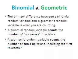
Binomial v. Geometric The primary difference between a binomial random variable and a geometric random variable is what you are counting. A binomial random variable counts the number of "successes" in n trials. A geometric random variable counts the number of trials up to and including the first "success."

Binomial vs. Geometric The Binomial Setting The Geometric Setting Each observation falls into one of two categories. The probability of success is the same for each observation. The observations are all independent. There is a fixed number n of observations. 4. The variable of interest is the number of trials required to obtain the 1st success. 1. Each observation falls into one of two categories. 2. The probability of success is the same for each observation. The observations are all independent.

FRQ Answers Must Include: Name of distribution Geometric, Binomial Parameters Binomial: X (define variable), n & p Geometric: X (define variable), p Probability Statement Ex: P (X = 7) or P (X 3) Calculation and p-value Calculator notation is okay, but needs to be labeled. Solution interpreted in context. 

Calculator: PDF PDF = precisely (exactly) a certain value Example: P (X = 2) TI 84: binompdf(n,p,r)TI 89: binomial Pdfn = number of trialsp = probability of successr = number of success

Calculator: CDF CDF = cumulative distribution. The probability of getting that value or something smaller. Example: P (X ≤3) TI 84: binomcdf(n,p,r)TI 89: binomial Cdfn = number of trialsp = probability of successr = number of success

Calculator: 1- CDF 1 – cdf = The probability of getting that value or something greater Example: P (X ≥ 8). 1 – bimoncfd (n-1, p, r)*** Must reduce n by 1, too***

Twenty-five percent of the customers entering a grocery store between 5 p.m. and 7 p.m. use an express checkout. Consider five randomly selected customers, and let X denote the number among the five who use the express checkout . What is the probability that two customers used the express check out?

Twenty-five percent of the customers entering a grocery store between 5 p.m. and 7 p.m. use an express checkout. Consider five randomly selected customers, and let X denote the number among the five who use the express checkout. hat is the probability that two customers used the express check out? Binomial Distribution N= 5 P = 0.25 X = # of people use expressP (X =2)

Twenty-five percent of the customers entering a grocery store between 5 p.m. and 7 p.m. use an express checkout. Consider five randomly selected customers, and let X denote the number among the five who use the express checkout . What is the probability that two customers used the express check out? binompdf (5, 0.25, 2) = .26375= number of customers0.25= probability of success2= number of successes desiredThere is a 26.37% chance that exactly 2 customers will use the express checkout lane between 5pm and 7pm.

Binomial & Normal The binomial distribution can be approximated well by a normal distribution if the number of trials is sufficiently large. A normal distribution can be used to approximate the binomial distribution if np is at least 10 and n(1-p) is at least 10.

Suppose we have data that suggest that 3% of a company’s hard disc drives are defective. You have been asked to determine the probability that the first defective hard drive is the fifth unit tested.

Suppose we have data that suggest that 3% of a company’s hard disc drives are defective. You have been asked to determine the probability that the first defective hard drive is the fifth unit tested. Geometric Distribution P = 0.03 X = # of disc drives till defective P (X = 5)

Suppose we have data that suggest that 3% of a company’s hard disc drives are defective. You have been asked to determine the probability that the first defective hard drive is the fifth unit tested. Geometpdf (0.03, 5) 0.03= p = probability of defect 5 = n= tests until defect foundP = 0.0266There is a 2.66% percent chance that the first defective hard drive is the fifth unit tested.