/
Wearable EMG System with Signal Compression and Decompression Wearable EMG System with Signal Compression and Decompression

Wearable EMG System with Signal Compression and Decompression - PowerPoint Presentation

pamela
pamela . @pamela
Follow
342 views
Uploaded On 2022-06-18

Wearable EMG System with Signal Compression and Decompression - PPT Presentation

Related reading Effective LowPower Wearable Wireless Surface EMG Sensor Design Based on AnalogCompressed Sensing Balouchestani amp Krishnan 2014 Sensors 14 2430524328 ID: 920524

signal norm amp compression norm signal compression amp 2014 krishnan balouchestani length sampling sparsity analog data signals compress number

Share:

Link:

Embed:

Download Presentation from below link

Download Presentation The PPT/PDF document "Wearable EMG System with Signal Compress..." is the property of its rightful owner. Permission is granted to download and print the materials on this web site for personal, non-commercial use only, and to display it on your personal computer provided you do not modify the materials and that you retain all copyright notices contained in the materials. By downloading content from our website, you accept the terms of this agreement.


Presentation Transcript

Slide1

Wearable EMG System with Signal Compression and Decompression

Related reading: Effective

Low-Power Wearable

Wireless Surface EMG

Sensor Design

Based on Analog-Compressed Sensing,

Balouchestani

& Krishnan

(

2014

).

Sensors

14: 24305-24328.

W. Rose 201704011

Slide2

Background

sEMG

signals exhibit

good level of sparsity in the time and frequency

domains.”

“Conventional data

acquisition approaches

rely

on the Shannon sampling

theorem, which

says

a signal must be sampled at least twice its bandwidth in order to be represented without error

.”

Sparse signal = a signal with most values zero or lacking information

Slide3

Drawbacks of conventional approach

Generates

huge intolerable

number of

samples for many applications with a large bandwidth.

Even

for low signal

bandwidths, including

some biomedical signals,

this produces

a large

number

of redundant digital samples.

Slide4

Cure

Use compressive sampling to reduce

the number of acquired samples by utilizing sparsity

.

Specifically, use analog compressive sampling before the analog-to-digital conversion step

Slide5

No compression

Digitize, then compress (more common than #3)

Compress, then digitize

Balouchestani

& Krishnan (2014)

Slide6

Question for the Authors

Balouchestani

& Krishnan (2014) say they apply compressive sampling to the

analog

signal before A-to-D conversion. (See bottom part of figure in previous slide.) But they implement their compression algorithm in computer code (C, hSpice

, or Matlab

). And their sample signals are from online databases. The fact that they implement in code (not with a circuit) and that their test data is already digitized means the ADC has already happened.

How do they account for this discrepancy?

How did they get it published?

Slide7

L-1 norm

The L1 norm is a way of measuring the “length of a vector” by the sum of the absolute values of its components.


Slide8

L-2 norm

The L2 norm is the Euclidean norm, in which we measure the length by the square

root of the

sum of the squares of the components.


Slide9

L

-

norm

The L-

norm means measuring the length of a vector by the length of it longest component.


Slide10

L-n norm

The L-n norm is a way of measuring the “length of a vector” by the n

th

root of the sum of the n

th power of each element.


Slide11

BSBL

Block-sparse Bayesian Learning

Slide12

Data Compression Examples

No

compression: standard audio

CD, .wav, .

aiff

Lossy

compression:

MP3, AAC Decompressed signal is not perfect, but very close

Typical compression factor = 4 to 20

Lossless compressed audio

formats

Decompressed signal is perfect copy

Typical compression

factor = 2

Codec Software or hardware to compress and decompress


Slide13

Transmitter and Receiver Design

Balouchestani

& Krishnan (2014)

Slide14

Eq

. 7

in

Balouchestani

& Krishnan (2014

) should be*

Sensitivity = % of “positives” that are correctly identified.

Specificity

= % of

“negatives

” that are correctly identified

.

T

P

= true positive;

F

N

= false negative, etc.* B.&K. 2014, eq.7, says:

Sens. = T

P

/ (T

P

+TN) (wrong)


Slide15

Step

7

of Table 2 in

Balouchestani

& Krishnan (2014) says sparsity level is given by

Sp

= (N/N-K)

w

hich is an unclear or wrong choice of parentheses, and K is undefined, and it is inconsistent with later figures, which show that Sparsity is a percentage that is 100% or less – which will not be true if computed with the equation above.

Slide16

Fig. 10 does not make sense. It indicates that the accuracy is highest when sampling rate is lowest, just 10% of the Nyquist rate.