Stable - PowerPoint Presentation

Slide1

Stable

Isotopes in Peat Profiles Reveal Long-term Carbon and Nitrogen Dynamics at SPRUCE Erik A. Hobbie1, Kirsten S. Hofmockel2, Karis J. McFarlane3, Colleen M. Iversen4, Janet Chen1, Nathan R. Thorp1, Paul J. Hanson41University of New Hampshire, 2Iowa State University, 3Lawrence Livermore National Laboratory, 4Oak Ridge National Laboratory

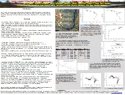
IntroductionPeat is a large reservoir of stored carbon and peat cores preserve a long-term record of system carbon and nitrogen dynamics. Stable isotopes are one marker of carbon and nitrogen dynamics in peat cores. Here, we investigated controls over δ15N and δ13C patterns in peat cores from the Marcell S1 forested bog in northern Minnesota.  Methods∙ Peat cores were collected in mid-August 2012 in 17 plots along 3 boardwalks extending out into bog S1 (Figure 1) using a modified hole saw (0-30 cm) or a Russian peat corer (30-250 cm depth).∙ Hollows were sampled to -250 cm and hummocks to -10 cm. Cores were sampled every 10 cm to 1 m; every 25 cm from 1-2 m, every 50 cm thereafter. Cores were taken in treed or non-treed locations. Mean depth of core sections is reported. ∙ Foliage, roots, and fungi were also sampled. ∙ δ15N and δ13C in samples were measured at the University of new Hampshire; radiocarbon was measured at Lawrence Livermore National Laboratory. ∙ δ13C patterns were analyzed using multiple regression in JMP with δ15N, %N, and %C as continuous variables and depth, plot location, topography (hummock or hollow), or vegetation (treed or non-treed) as nominal variables. δ15N was analyzed using the same variables and δ13C.∙ δ13C and δ15N were also correlated against radiocarbon (∆14C).Results∙ δ13C was lowest in hummocks (above 0 cm) and then increased by 3‰ to -85 cm (Figure 2a).∙ δ15N was lowest in hummocks and increased by up to 6‰ to -35 cm before declining (Figure 2b).∙ The log C/N steadily declined to around 3 at -85 cm (C/N = 20) (Figure 2c).∙ In multiple regression analyses, δ15N and δ13C correlated strongly with depth, plot location, %C, %N, and each other, with δ13C also correlating with topography (Table 1). The models explained 85% and 74% of variance for δ13C and δ15N. ∙ Depth accounted for <50% of variance and the depth coefficients for δ13C and δ15N correlated strongly (Figure 3).∙ Plot location accounted for <15% of variance and the plot coefficients for δ13C and δ15N correlated negatively (Figure 4a), with high δ15N and low δ13C coefficients in the western lagg zone closer to uplands (Figure 4b).∙ Patterns in δ15N and δ13C against radiocarbon (Figure 5a and 5b) were used to link stable isotopes to specific time periods. Discussion/Conclusions ∙ The negative correlation of δ15N with %N (Table 1) could reflect either removal of 15N-enriched N or addition of 15N-depleted N, possibly via N fixation. The increase in the depth coefficient for δ15N of ~3‰ from -25 cm to -35 cm (Figure 3) suggested that the N removal process primarily operates at a discrete depth, presumably corresponding to the juncture between aerobic and anaerobic layers defined by the water table. ∙ Higher δ15N and lower δ13C in plots closer to uplands (Figure 4b) may reflect distinct hydrology and accompanying shifts in C and N dynamics in the lagg area. ∙ The Suess effect and aerobic decomposition lowered δ13C in recent surficial samples. ∙ Small increases in δ13C at -112 cm (4290 calibrated years BP) and -85 cm (3820 calibrated years BP) may reflect C dynamics during a suspected transitional fen stage (based on paleoecology at a nearby bog, Verry and Janssens 2011), with reduced methanotrophy during this period retaining less 13C-depleted carbon derived from methane than in later periods. ∙ This may reflect a phase during which sedges transported methane directly to the atmosphere, thereby minimizing the refixation in Sphagnum cells of 13C-depleted, methanotrophic-derived carbon dioxide.∙ A peak in δ13C and trough in δ15N at -400‰ ∆14C (4220 calibrated years BP, Figure 5) suggests that processes increasing δ13C such as high sedge abundance may decrease sequestration of 15N-enriched organic matter. ∙ We are currently exploring whether climate can be linked to these isotopic shifts and whether isotopic modeling will provide further insights into C and N dynamics at S1 during the Holocene.Referencess: Verry ES, Janssens J. 2011. Geology,vegetation, and hydrology of the S2 bog at the MEF: 12,000 years in northern Minnesota. RK Kolka, Peatland Biogeochemisty and Watershed Hydrology at the Marcell experimental Forest: 93-135.

Acknowledgements

The authors appreciate field sampling

by members of the SPRUCE research group, in particular Jana Phillips and Deanne Brice. This material is based upon work supported in part by the U.S. Department of Energy, Office of Science, Office of Biological and Environmental Research. Oak Ridge National Laboratory is managed by UT-Battelle, LLC, for the U.S. Department of Energy under contract DE-AC05-00OR22725. DOE grant ER65430 to Iowa State University also supported this work. The data referenced here are archived at and available from the SPRUCE long-term repository (http://mnspruce.ornl.gov).

Figure 1. Aerial photograph of the S1 bog (23 September 2014) showing the 17 experimental plots (each 10.4 m in diameter to the outer edge of the visible perimeter boardwalk). Plot numbers on the image represent the plot areas within which peat was sampled.

Table

1. Regression model for explaining δ13C and δ15N in peat profiles at SPRUCE. Vegetated vs non-vegetated, hummock vs. hollow topography. Plot and depth treated as nominal variables. Value = Coefficient ± standard error; Var. = % variance explained. n = 219. δ13C model, adjusted r2 = 0.853, p <0.001 δ15N model, adjusted r2 = 0.738, p <0.001Source Value±SE %Var. P Source Value±SE %Var. P Intercept -30.68±1.14 -- -- Interc 33.41±4.47 -- --δ15N 0.18±0.03 14.4 <0.001 δ13C 0.74±0.14 9.7 <0.001%N 0.366±0.141 3.4 0.010 %N -1.061±0.277 5.0 <0.001%C 0.066±0.024 3.9 0.006 %C -0.235±0.045 9.1 <0.001Vegetated -0.07±0.07 0.6 0.287 Veg 0.12±0.14 0.3 0.367Hummock 0.29±0.12 1.9 0.056 Humm 1.11±0.29 4.8 <0.001Plot -- 16.7 0.008 Plot -- 17.8 <0.001Depth -- 59.2 <0.001 Depth -- 53.3 <0.001

Figure 3

. Depth coefficients of δ15N and δ13C from regression models correlate in peat profiles. The depth in cm is indicated next to coefficients (±SE).

Figure

4a. Plot coefficients of δ15N and δ13C from regression models correlate in peat profiles. Standard error bars omitted for clarity, and averaged 0.24‰ for δ15N and 0.12‰ for δ13C. The plot number is the symbol for the paired coefficient values. Data plotted below, equation, δ15N = -1.37±0.57 × δ13C + 0.00±0.10, adjusted r2 = 0.243, p = 0.030.

Figure 5b.

Relationship between ∆

14

C and δ13C.

Figure 2

. δ

15

N, δ13C, and log C/N versus depth (Figure 2a, 2b, and 2c). Values (±SE) are averaged across hummock versus hollow cores and across treed versus non-treed cores. Averages (±SE) are given for each depth, with n given in parentheses following the depth: 25 cm (3), 22 cm (7), 14 cm (14), 5 cm (14), -5 cm (19), -15 cm (17), -25 cm (17), -35 cm (15), -45 cm (17), -55 cm (17), -65 cm (17), -85 cm (18), -112 cm (17), -162 cm (17), -210 cm (1), -225 cm (8), -260 cm (1).

Figure 5a. Relationship between ∆14C and δ15N.

Figure 4b. Plot coefficients of δ15N and δ13C showing the spatial relationship among coefficient values. Plot locations as given as in Figure 1, with plot 4 at lower left. Values are given × 10 for the δ15N and δ13C coefficients, as (δ15N, δ13C). Coefficients are color-coded, with blue = high δ15N, red = low δ15N, and purple intermediate δ15N.

Figure 2b

Figure 2c

Figure 2a