/
http://projecteuclid.org/euclid.aoas/1458909913 http://projecteuclid.org/euclid.aoas/1458909913

http://projecteuclid.org/euclid.aoas/1458909913 - PowerPoint Presentation

pasty-toler
pasty-toler . @pasty-toler
Follow
382 views
Uploaded On 2017-09-15

http://projecteuclid.org/euclid.aoas/1458909913 - PPT Presentation

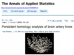
The full data set consists of n 98 or 97 such trees from people whose ages range from 18 to 72 years old Each data point is a tree representing arteries in human brains isolated via magnetic resonance imaging ID: 587979

add siblings kill http siblings add http kill parent https youngest org www persistence baby test html data trees bubenik15a csbsju physics

Share:

Link:

Embed:

Download Presentation from below link

Download Presentation The PPT/PDF document "http://projecteuclid.org/euclid.aoas/145..." is the property of its rightful owner. Permission is granted to download and print the materials on this web site for personal, non-commercial use only, and to display it on your personal computer provided you do not modify the materials and that you retain all copyright notices contained in the materials. By downloading content from our website, you accept the terms of this agreement.


Presentation Transcript

Slide1

http://projecteuclid.org/euclid.aoas/1458909913

Slide2

The full data set consists of n = 98 (or 97) such trees from people whose ages range from 18 to 72 years old.

Each data point is a tree (representing arteries in human brains isolated via magnetic resonance imaging), embedded in

3-dimensional space, with additional attributes such as thickness (ignored).

These diagrams are turned into feature vectors:

(p

1

, p

2

, …, p

100

) where p

i

is the length of the

i

th

longest for for H

0.

(q

1

, q

2

, …, q

100

) where q

i

is the length of the

i

th

longest for for H

1.

Slide3

0 1 10

Why use PCA?

Consider the points (0, 0, …, 0), (1, 0, …, 0), (10, 0, …, 0)

Add noise to first point (0, 0, …, 0)

 (0, 1, …, 1)

In R

100

, d(

(0, 1, …, 1)

, (1, 0, …, 0)) = 10 > 9.

Add small noise to first point (0, 0, …, 0)

 (0, 0.1, …, 0.1)

In R

39,900

, d(

(0, 0.1, …, 0.1)

, (1, 0, …, 0)) = 20 > 9.

Slide4

http://jmlr.csail.mit.edu/papers/volume16/bubenik15a/bubenik15a.pdf

Slide5

from: https://www.cs.montana.edu/brittany/research/docs/fasy_socg2014_slides.pdf

Slide6

http://jmlr.csail.mit.edu/papers/volume16/bubenik15a/bubenik15a.pdf

Slide7

Figure 6: We sample 1000 points for a torus and sphere, 100 times

each,

mean persistence landscape in dimension 0, 1 and 2

http://jmlr.csail.mit.edu/papers/volume16/bubenik15a/bubenik15a.pdf

Slide8
Slide9

https://en.wikipedia.org/wiki/Neuron#/media/

File:Blausen_0657_MultipolarNeuron.png

Slide10

From "Texture of the Nervous System of Man and the Vertebrates" by 

Santiago Ramón y

Cajal

. The figure illustrates the

diversity of


neuronal

 morphologies in the 

auditory cortex

.

http://

thebrain.mcgill.ca/flash/a/a_01/a_01_cl/a_01_cl_ana/a_01_cl_ana.html

http://

www.mind.ilstu.edu/curriculum/neurons_intro/neurons_intro.php

Slide11
Slide12

z

(v, f)

(1, 1.5)

(

1. 2)

Start with all the leaves:

A = {a

1

, z

1.5

, c

3

, e

4

, g

5

, h

6

}

a

1

youngest.

A contains all siblings of a

1.

Kill a

1

and all its siblings.

Add parent of a

1.

A = {b

3

,

e

4

, g

5

, h6} Slide13

z

(v, f)

(1, 1.5)

(

1. 2)

(

5, 4)

Start with all the leaves:

A = {a

1

, z

1.5

, c

3

, e

4

, g

5

, h

6

}

a

1

youngest.

A contains all siblings of a

1.

Kill a

1

and all its siblings.

Add parent of a

1.

A = {b

3

,

e

4

, g

5

, h

6

}

ignore b

2

and

e

4

since siblings

not in A.

g

5

youngest with all siblings in A.

Kill g

5

and all its

siblings. Add

parent of

g

5

.

A = {

b

3

,

e

4

,

f

6

}

Slide14

z

(v, f)

(1, 1.5)

(

1. 2)

(

5, 4)

(

4, 3)

Start with all the leaves:

A = {a

1

, z

1.5

, c

3

, e

4

, g

5

, h

6

}

a

1

youngest.

A contains all siblings of a

1.

Kill a

1

and all its siblings.

Add parent of a

1.

A = {b

3

,

e

4

, g

5

, h

6

}

ignore b

2

and

e

4

since siblings

not in A.

g

5

youngest with all siblings in A.

Kill g

5

and all its

siblings. Add

parent of

g

5

.

A = {

b

3

,

e

4

,

f

6

}

e

4

youngest with all siblings in A

.

Kill e

4

and all its

siblings.

Add parent of

b

2

.

A = {

b

3

, d

6

}

Slide15

z

(v, f)

(1, 1.5)

(

1. 2)

(

5, 4)

(

4, 3)

(

3, 2)

Start with all the leaves:

A = {a

1

, z

1.5

, c

3

, e

4

, g

5

, h

6

}

a

1

youngest.

A contains all siblings of a

1.

Kill a

1

and all its siblings.

Add parent of a

1.

A = {b

3

,

e

4

, g

5

, h

6

}

ignore b

2

and

e

4

since siblings

not in A.

g

5

youngest with all siblings in A.

Kill g

5

and all its

siblings. Add

parent of

g

5

.

A = {

b

3

,

e

4

,

f

6

}

e

4

youngest with all siblings in A

.

Kill e

4

and all its

siblings.

Add parent of

b

2

.

A = {

b

3

, d

6

}

Kill

b

3

and all its siblings

.

Add parent of b

2

.

A = {R} Slide16

z

(v, f)

(1, 1.5)

(

1. 2)

(

5, 4)

(

4, 3)

(

3, 2)

(6, 0)

Start with all the leaves:

A = {a

1

, z

1.5

, c

3

, e

4

, g

5

, h

6

}

a

1

youngest.

A contains all siblings of a

1.

Kill a

1

and all its siblings.

Add parent of a

1.

A = {b

3

,

e

4

, g

5

, h

6

}

ignore b

2

and

e

4

since siblings

not in A.

g

5

youngest with all siblings in A.

Kill g

5

and all its

siblings. Add

parent of

g

5

.

A = {

b

3

,

e

4

,

f

6

}

e

4

youngest with all siblings in A

.

Kill e

4

and all its

siblings.

Add parent of

b

2

.

A = {

b

3

, d

6

}

Kill

b

3

and all its siblings

.

Add parent of b

2

.

A = {R} Slide17

Mathematical random trees are defined by a set of parameters that constrain their shape:

We defined a control group as a set of trees generated with predefined parameters

Accuracy if vary 1 parameter:Slide18

dBar: For each barcode we generate a density profile

as follows:

For all x in

R,

the value of the histogram

is the number of intervals that contain x , i.e., the number of components alive at that point.

The distance between two barcodes D (T1) and D (

T ) is defined as the sum of the differences between the density profiles

of the barcodes

.

This distance is not stable with respect to

Hausdorff

distance, but it is the only distance we are

aware of

that succeeds in capturing the

differences

between

distinct neuronal

persistence barcodes.Slide19
Slide20
Slide21

http://neuromorpho.org/

Slide22
Slide23

Topological

comparison of neurons from different animal species. Each

row corresponds

to a species: (I) cat, (II) dragonfly, (

III) drosophila

, (IV) mouse and (IV) rat

.

Note that the trees, barcodes, and persistent images are not shown to the same

scaleSlide24

https://

arxiv.org/abs/1507.06217

Abstract

Many datasets can be viewed as a noisy sampling of an underlying topological space.

Topological

data analysis aims to understand and exploit this underlying structure for the

purpose of

knowledge discovery. A fundamental tool of the discipline is persistent homology, which

captures underlying data-driven, scale-dependent homological information. A representation in

a "persistence diagram" concisely summarizes this information. By giving the space of persistence diagrams a metric structure, a class of effective machine learning techniques can be applied.

We modify

the persistence diagram to a "persistence image" in a manner that allows the use of

a wider

set of distance measures and extends the list of tools from machine learning which can

be utilized

.

It is shown that several machine learning techniques, applied to persistence images

for classification

tasks, yield high accuracy rates on multiple data sets. Furthermore, these

same machine

learning techniques fare better when applied to persistence images than when

applied to

persistence diagrams. We discuss sensitivity of the classification accuracy to the

parameters associated

to the approach. An application of persistence image based classification to a data

set arising

from applied dynamical systems is presented to further illustrate.Slide25

b

x

= birth, b

y

= death,

b

= death - birth

https://

en.wikipedia.org/wiki/Gaussian_function

https://

arxiv.org/abs/1507.06217

Slide26

Topological

comparison of neurons from different animal species. Each

row corresponds

to a species: (I) cat, (II) dragonfly, (

III) drosophila

, (IV) mouse and (IV) rat

.

Note that the trees, barcodes, and persistent images are not shown to the same

scaleSlide27

Apical dendrite trees

extracted from several types of rat neuron

. From these persistent

images we train a decision tree classifier on

the expert-assigned

groups of cells. Slide28
Slide29
Slide30
Slide31
Slide32

If all c

i

= 1 and all m

i

are different, then barcode can be determined from APF.Slide33
Slide34
Slide35

https://www.lebesgue.fr/sites/default/files/attach/

Biscio.pdf

Slide36
Slide37
Slide38
Slide39
Slide40
Slide41
Slide42
Slide43

Kolmogorov-Smirnov TestSlide44

Sorted

controlB={0.08, 0.10, 0.15, 0.17, 0.24, 0.34, 0.38, 0.42, 0.49, 0.50, 0.70, 0.94, 0.95, 1.26, 1.37, 1.55, 1.75, 3.20, 6.98, 50.57}

http://www.physics.csbsju.edu/stats/KS-test.html

Slide45

Sorted

controlB={0.08, 0.10, 0.15, 0.17, 0.24, 0.34, 0.38, 0.42, 0.49, 0.50, 0.70, 0.94, 0.95, 1.26, 1.37, 1.55, 1.75, 3.20, 6.98, 50.57}

http://www.physics.csbsju.edu/stats/KS-test.html

Slide46

treatmentB

= {2.37, 2.16, 14.82, 1.73, 41.04, 0.23, 1.32, 2.91, 39.41, 0.11, 27.44, 4.51, 0.51, 4.50, 0.18, 14.68, 4.66, 1.30, 2.06, 1.19}

http://www.physics.csbsju.edu/stats/KS-test.html

Slide47

treatmentB

= {0.11, 0.18, 0.23, 0.51, 1.19, 1.30, 1.32, 1.73, 2.06, 2.16, 2.37, 2.91, 4.50, 4.51, 4.66, 14.68, 14.82, 27.44, 39.41, 41.04}

http://www.physics.csbsju.edu/stats/KS-test.html

Slide48

The KS-test uses the maximum vertical deviation between the two curves as the statistic D. In this case the maximum deviation occurs near x=1 and has D=.45. (The fraction of the treatment group that is less then one is 0.2 (4 out of the 20 values); the fraction of the control group that is less than one is 0.65 (13 out of the 20 values). Thus the maximum difference in cumulative fraction is D=.45.)

http://www.physics.csbsju.edu/stats/KS-test.html

Slide49
Slide50

False Positives will occur

https://xkcd.com/882

/

Slide51

http://blog.minitab.com/blog/adventures-in-statistics-2/how-to-correctly-interpret-p-

values

Example: vaccine

study

with

P value of 0.04

:Correct: Assuming that the vaccine had no effect, you’d obtain the observed difference or more in 4% of studies due to random sampling error.

Incorrect: If you reject the null hypothesis, there’s a 4% chance that you’re making a mistake.Slide52

But there likely are gender differences:

From: http://www.parenting.com/article/harder-to-raise-boys-or-girls

In a nutshell, girls are rigged to be people-oriented, boys to be action-oriented

.

From:

http://scicurious.scientopia.org/2011/03/09/baby-boy-baby-girl-baby-x

/

Baby girls are treated as more delicate than baby boys, and baby boys get more attention for gross

motor …. Not only that, mothers TOUCH male infants more initially than they do female infants, though this trend reverses at 6 months of age, and they verbalize to female infants more.

Sidorowicz, L., & Lunney, G. (1980). Baby X revisited Sex Roles, 6 (1), 67-73 DOI: 10.1007/BF00288362

Seavey

, Katz, and

Zalk

(1975). Baby X: The effect of gender labels on adult responses to infants Sex roles, 1 (2)Slide53

https://arxiv.org/format/

1608.03520

In

this network, nodes correspond to 83 brain regions

defined

by the Lausanne

parcellation

[26] and edges

correspond to the density of white matter tracts between node pairsSlide54
Slide55

http://www.nature.com/neuro/journal/v20/n3/full/nn.4502.

html

Slide56

https://en.wikipedia.org/wiki/Neuron#/media/

File:Blausen_0657_MultipolarNeuron.png

Slide57

https://en.wikipedia.org/wiki/Axon#/media/File:Neuron_Hand-

tuned.svg

Slide58

The tissue called "gray matter" in the brain and spinal cord is made up of cell bodies.

"White matter” is composed of nerve fibers (axons).

https://medlineplus.gov/ency/imagepages/18117.

htm

Slide59

https://www.ncbi.nlm.nih.gov/pmc/articles/PMC2768134

/

Slide60

https://arxiv.org/format/

1608.03520

In

this network, nodes correspond to 83 brain regions

defined

by the Lausanne

parcellation

[26] and edges

correspond to the density of white matter tracts between node pairsSlide61