PPT-A Comparison of Two Volcanic Ash Height PowerPoint Presentation

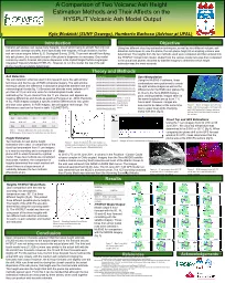
Estimation Methods and Their Affects on the HYSPLIT Volcanic Ash Model Output Kyle Wodzicki SUNY Oswego Humberto Barbosa Advisor at UFAL Conclusion References

Upload by phoebe-click
Published on 2016-06-15

Presentation Embed Code

<iframe width="560" height="315" src="https://www.docslides.com/embed/363545" frameborder="0" allowfullscreen></iframe>

Download Presentation

Download Presentation The PPT/PDF document "A Comparison of Two Volcanic Ash Height" is the property of its rightful owner. Permission is granted to download and print the materials on this web site for personal, non-commercial use only, and to display it on your personal computer provided you do not modify the materials and that you retain all copyright notices contained in the materials. By downloading content from our website, you accept the terms of this agreement.