/
Proceedings IROS  Conference on Intelligent Robots and Systems Takamatsu Japan Planning Proceedings IROS  Conference on Intelligent Robots and Systems Takamatsu Japan Planning

Proceedings IROS Conference on Intelligent Robots and Systems Takamatsu Japan Planning - PDF document

phoebe-click
phoebe-click . @phoebe-click
Follow
562 views
Uploaded On 2014-12-12

Proceedings IROS Conference on Intelligent Robots and Systems Takamatsu Japan Planning - PPT Presentation

This paper presents a planning and control methodology for such systems allowing them to follow simultaneously desired endeffector and platform trajectories without violating the nonholonomic constraints Based on a reduction of system dynamics a mod ID: 22735

This paper presents

Share:

Link:

Embed:

Download Presentation from below link

Download Pdf The PPT/PDF document "Proceedings IROS Conference on Intellig..." is the property of its rightful owner. Permission is granted to download and print the materials on this web site for personal, non-commercial use only, and to display it on your personal computer provided you do not modify the materials and that you retain all copyright notices contained in the materials. By downloading content from our website, you accept the terms of this agreement.


Presentation Transcript

Mobile manipulator comprised of a mobile with one or more manipulators, are of great interest in a numberof applications. This presents a planning platform trajectoriesBased on areduction of system dynamics, a model-based controller isdesigned to eliminate tracking sensitivity to parameter errors is examined andfound to be validity of methodology is1IntroductionMobile manipulator systems consist of a mobile Applications forabound in Manipulator Fig. 1.Mobile manipulator system.A host of issues related to studied in application, control in thepresence of base see for example [1-4]. However, in these studies, the mobilesubject to nonholonomicplanning for mobile platforms is open loop controls which steer the platform from an state to a final one, without violating the nonholonomicconstraints, see for example [5-6]. The emphasis a. Differential-Drive Mobile Manipulator =0.30mb=0.30mr=0.10m=0.30m=0.15m=0.35m=0.12m 11l1I1m1 bl21l2 2m2GFE 0m0 xF,yF)(xE,yE) ManipulatorDrivenWheelDrivenWheel Y The platform moves by driving the two as shown in the figure. On the assumption of low wheels do not sideways. TheeúsinúcosúxylFFGjjj-+=0(1)and F. It can be see [5], [6], that Eq. (1) is a nonholonomic constraint i.e. aFocusing on the platform first, the relating the wheel rates to the ú j, is jjjjjjjj and are the angular velocities of the left and respectively and the symbols c and s have used instead of sin. The two angular velocities aremapped to system velocities. Furthermore, inmobile platforms, this type of Keeping the first two equations in matrix Eq. (2) and 0, i.e. if themanipulator is mounted on the axis that connects the centers, then the second matrix in Eq. (3) becomes all points along this axis must perpendicular to freedom is lost. Mounting the manipulator The linear velocity of the effector is found base velocity is known given by Eq.11122122, are and y components of the velocityof E, and (i, j = 1,2) terms the elements of theJll1111212=--+sin()sin()JJJ12212=-+sin()Jll2111212=++cos()cos()JJJ22212cos(), are the lengths of the upper arm, and the, are variables of ú , is still in Eq. (4), as an input term. By writing the rate in terms of the wheel rates, combining Eqs. (3) (4), the////()/()/rJrbrJrbJJlJrblJrbJJ-++2201111111221212122lrblrbúúúxRJvJvb.Car-like Mobile Manipulatorconsider a simple mobile manipulator system includes a Fig. 3.The rear wheels are parallel to the main axis of the car whilethe front wheel is used for steering the platform. Again, the =0.30m=0.15m=0.35m=0.12m=0.30mb=0.30mr=0.10ml=0.5m 11l1bl21l2 xE,yE) ManipulatorWheelDrivenWheel F 0m0(xF,yF) Y For simplicity, the manipulator is mounted at point F,where the steering wheel is also. For this point the xyljjj-+=0(7) are the x and y components of the velocity of point F respectively, is the kinematics of the cos()sin() is the steering angle, is the velocity due is the front wheel angular is its radius. The zero column of the matrix in Eq. (8)shows that if the mobile platform is not moving (then neither the position nor the orientation of the platformEq. (8) is in a form its Jacobian contains a zero column. To solve this problem,Note that this change of input velocities gives a form that is always invertible. As for the 11122122Jij(,,)12 are defined in Eqs. (5).Next, the platform rotation is substituted usingline of the matrix Eq. (8) while the resultingequation is appended to Eq. (9) to yield JJr000000111211212221xRJJ corresponds to the last column vector in Eq. The task we tackle in this section is to inputs so that the platform follow given trajectories. A typical application forthis problem is the robotic crack-sealing, where a mobile platform is required to follow a given path, (11) can be used to generate velocities so that the platform s end-the nonholonomic constraints,result in motions that do notviolate the nonholonomic constraint therefore areachievable by the mobile manipulator system. The platform ú is found using the last equation in Eq.(2) or Eq. (8). The platform orientation is found byintegrating this angular velocity. We assume that the crack to follow is available. Setting some time inwhich the task must be results in the curve followed by the point F on the either is arbitrarily specified on the condition that the) and (x) is within the reach ofthe manipulator, or corresponds to a prescribed path forwhich the same condition follows. Otherwise, the task isand a Indeed, the lllr00180detsin,llr00180which means that a singularity arises when the manipulatorextended or folded. Indeed, in location for E is reach of and a tool at E cannot follow the can be overcome by re-planning the path of F.Moreover, it is advantageous to choose the motion of F so that it is smooth and that its curvature does not violateAlthough the inversion of the kinematic wheel rates, one has to control such amobile manipulator system by applying the that will eliminate any should take into the mass properties of the mobileTherefore, in the next section we derive the4Dynamics of the Differential-Drive Mobiles equations of dynamics of mechanical systems subject tooThe system under consideration is subject to a singlenonholonomic constraint, which is described by 0(14)()sincoscosjjlG00úúúúúúq=[]xyFFTjJJTo derive equations of for the mobilemanipulator system, first let represent theAssuming that the massthe moments of inertia of the 4 LmxyJmxyJmxyJGGAA=++++++++++++212jJjJJ are the masses and the momentsof inertia of the platform, the first xyxyxyGGAABB the x, components of the velocities of the center of mass of theforces as input terms forms theequations of motion of the not allowing the wheels to Aq0-+-==xyFFTjJJcorresponds to represents forces. The columns of form a non-normalized base forExpressing Eq. (15) in terms of the substituting the result into Eq. (16), theMqqVqqEqAq)()()+=- t () is the 5Vqq) is the of velocity-dependent tt tttt,,, is the 4-() is a 54 input is the Lagrange multiplier.Eq. (14) shows that the constraint velocity is always inthe nullspace of (), so it is possible to to nnnn1234 such thatqSqv() contains the base vectors of the. The selection of the base of the is important and allows the independent velocities to () to be lrslrslrclrcrbrb00100001of rank 4 since det()=(1+l)r/b0vector ofúúúúúJJJJDifferentiating Eq. (18), substituting the expression for úú into Eq. (17) and premultiplying by SMSvMSvVSE tt Note that since (), vanishes from theMvVE*** t MSMSVSMSvV, and ESE, i.e. the identity 44 matrix. Since is non- is always symmetricEq. (21) can be transformed further in MxVFJ+== tt MJMJ and contains all the velocityterms. Eq. (22) is in a very useful form because it links the5Model-based Control DesignEq. (22) is in the form of holonomic can be control of the tt JMxVúúúú)()xxKxxKxx=+-+-dvdPdIn Eq. (24), the subscript corresponds to vviPpidiagkdiagk{},{}substituting Eq.(24) into Eq. (23), and applying the resulting torques to theúúúekekeivipi++=0, i = 1,,4(25)exxiidi. These equations, which linear andpermit the selection of the elements of the gain and so as to have tt JMxV M represent the estimates of the terms in thedynamical model. Using Eq. (26) as a nonlinear control lawúúúeKeKed dIJMJMxJMJVV()(()(TTTTdescribed by Eq. (27) is nonlinear error convergence is ensured due to two mobile manipulatorsshown in Figs. 2 and 3 are parameters are displayed in the same figures. For motion time was equal to 6s(so as to ) = (0.5m, , -30). The final positions ) = (2m, -2m, 1.9m, -1.9m). Thepoint F on the mobile platform was using a third order polynomial for the time ). The given4. Figs. 5 and 6 present snapshots of the motion of the 00.511.522.5 Fig. 4.Desired platform and end-effector paths. 0 00.5 Fig. 5.Animation of the motion of the mobilemanipulator with a differential drive. 00.511.52 the cusp that appears in those figures takes in different can bethat the cusp of the manipulator is sharper than that of the one. This isnot surprising as the system has theNext, we apply the control algorithm to themobile manipulator using the trajectories in Section 6a. The system mass properties areTable I.Mobile manipulator mass propertiesParameterValue 50.0kg 4.0kg3.5kg1.417kg m0.030kg m0.036kg mselected to force exhibit a critical response with a settling time equal to 1 s.12 and Fig. 7 shows the torques applied on torques applied on the joints of theend-effector andeliminated by the controller, 012345678 Fig. 7.Driving wheel torques. 012345678 Fig. 8.Manipulator torques. If the values of the kinematics not known, the controller is valid, on the condition of small uncertainties. This isillustrated in uncertainties ofthe order of 3-5% were introduced. In Fig. 9, the history ofF of the platform shown for an 8s runtime for thesame initial error as before. It can be seen errors converge to zero, although their responses from the ones where system known. Figs. 9and 10 depict the resulting joint and wheel torques, xE_err (m) 0.030.04 0246802468 0246802468 0.030.04-0.0050.010.0150.020.0250.03Fig. 9.Errors with parameter uncertainties. 0123456 Fig. 10.Driving wheel torques with uncertainties. 012345678 Fig. 11.Manipulator torques with uncertainties.7Conclusionspaper focused on control ofmobile manipulators, using as examples a system. Both system platforms with a two link manipulator. The kinematics for the two mobile written so asto map platform velocities to velocities, without violation of the nonholonomicspecification of trajectories forboth the platform computation ofactuator commands. Orthogonal complements and thewere used to equations of Based on controller wasdesigned to eliminate tracking errors. The controller wassuccessfully to a simple controller was shown to be [1]Papadopoulos, E. A New Measure offor Mobile Manipulators,Proc. IEEE Int. Conf. on Robotics [2]Papadopoulos, E. A FrameworkTask Planning of Mobile Vol. 16, No.[3]Hootsmans, N. A. Motion Control of Mobile Manipulators Conference on [4]Wiens, G., J., Effects of Dynamic Coupling inMobile Robotic Systems,Gaithersburg, MI, May[5]Lafferiere G. and for Controllable Systems without Drift,Conference on [6]Murray R. and Sastry S. S., Panning: Steering using Sinusoids,Trans. on, Vol. 38, No. 5, May[7]Kolmanovsky I. and McClamroch, H., in Nonholonomic Control Problems,[8]Seraji H., A Unified Approach to of Mobile Manipulators,Int. J. Robotics [9]Lim D. Configuration Control of atation and Experimentation,Int. J. Robotics Robotics Saha K. S. Dynamics ofSystems using a ASME J. of Sarkar N, Control ofSystems with Rolling Constraints:Application to Dynamic Control of Mobile Robots,Int. J. Robotics , Vol. 13, No. 1, t x