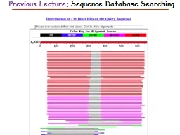
Previous Lecture: Sequence Database Searching - PowerPoint Presentation

Slide1

Previous Lecture:

Sequence Database Searching

Slide2

Introduction to Biostatistics and Bioinformatics

Distributions

This Lecture

By Judy Zhong

Assistant Professor

Division of Biostatistics

Department of Population Health

Judy.zhong@nyumc.org

Slide3

IntroductionLast lecture defined probability and introduced some basic tools used in working with probabilities

This lecture discusses specific probability models Three specific probability distributions (models) Binomial distribution Poisson distributionNormal distribution

3

Slide4

Random variablesA

random variable is a function that assigns numeric values to different events in a sample space NOTE: (1) Randomness; (2) Numeric valuesExample 1:

Randomly select a student from a class. X=student’s number of siblings. X could be 0, 1, 2 …Example 2: Randomly select a student from a class. X=student’s height. X could be any value bigger than 0

4

Slide5

Two types of random variables

A random variable for which there exists a discrete set of numeric values is a discrete random variableA random variable whose possible values cannot be enumerated is a continuous random variable

5

Slide6

Probability distribution functionA

probability distribution function is a mathematical relationship, or rule, that assigns to any possible value r of a discrete random variable X the probability Pr(X=r). 6

Slide7

Expected value (expectation) of a discrete random variable The

expected value (expectation) of a discrete random variable is defined asWhere x_i’s are the values the random variable X assumes with positive probabilityThe sum is over all the R possible values. R may be finite (e.g., binomial distribution) or infinite (e.g., Poisson distribution)Expectation represents “average” value of the random variable

7

Slide8

Variance (population variance) of a discrete random variable The

variance of a discrete random variable is defined byThe standard deviation of a random variable is defined by

8

Slide9

An experiment (for binomial distribution) Common structure for binomial distribution:

A sample of n independent trialsEach trial can have only two possible outcomes, which are denoted as “success” and “failure” (the term “success” is used in a general way, without specific meaning)The probability of a success at each trial is assumed to be the same, with probability p (hence the probability of failure is 1-p=q)

Let random variable: X=number of successes among n trails

9

Slide10

How to fit a real problem into binomial structureHere we concentrate on counting the number of neutrophils of 5 white blood cells.

Assume that the probability that a cell is neutrophils is 0.6number of trials n=5“success”=“one cell being neutrophils”Pr(“success”)=p=0.6X=number of successes among 5

10

Slide11

How to calculate the probability of an outcome from binomial structure There are 5 white cells, each of cell is either neutrophils (N) or other (O). What is the probability that the 2

nd and the 5th cells considered will be neutrophils and the remaining cells are non-neutrophils? That is, what is the probability of outcome “ONOON”Assume that the outcomes for different cells are independent. Using multiplication law of probability, Think about this question: What is the probability that any 2 cells out of 5 will be neutrophils?

11

Slide12

Combination plays an role …Possible outcomes for 2 neutophils of 5 cells:

NNOOO, ONNOO, …How many such outcomes? Then the probability of obtaining 2 neutrophils in 5 cells is:

12

Slide13

Binomial distributionLet

X=number of success in n statistically independent trials, where the probability of success is pThe distribution of random variable X is known as the binomial distribution and has probability distribution function given by

13

Slide14

Using binomial tablesTable 1 in the Appendix:

for n=2, 3, …, 20 and p=0.05, 0.10, …, 0.50

14

Slide15

Expected value and variance of the binomial distributionResult:

The expected value and the variance of a binomial distribution are np and np(1-p), respectively

15

Slide16

Bernoulli distribution

16Look at a special case of binomial random variable with n=1 and p. That is, conduct only one trial, X=1 if success and X=0 if failure:

Pr(X = 1) =pPr(X = 0) = 1 − p = qExpectation of X: E(X)=1*p+0*q=p

Variance of X: Var(X)=(1^2*p+0^2*q)-p^2=p*(1-p)=pq

Slide17

Write binomial random variable in terms of bernoulli random variablesConduct n independent trials, each trail having outcome either success or failure

For each trail, probability of success is pX=number of successes among n trials. It is known that the distribution of X is binomial distribution with n and pNow define the outcome of the ith trial as Xi (Xi=1 if success and Xi=0 if failure), then

17

Slide18

Proof of expectation and variable of binomial variable Fact 1:

Fact 2: For any i, E(Xi)=p and Var(Xi)=pqThen (1) , where the first equality always holds(2) , where the first equality only holds for independent variables

18

Slide19

Poisson distribution for rare eventsThe Poisson distribution is the second most frequently used discrete distribution after the binomial distribution. Poisson distribution is usually associated with rare events (for example, rare diseases)

19

Slide20

Examplesnumber of deaths attributed to typhoid fever over a year

Assuming the probability of a few death from typhoid fever in any one day is vey small and the number of cases reported in any two days are independent random variables, then the number of deaths over a 1-year period will follow a Poisson distributionnumber of bacterial colonies growing on an agar plate.Suppose we have a 100-cm^2 agar plate. The probability of finding any bacterial colonies on a small area is very small, and the events finding bacterial colonies at any two areas are independent. The number of bacterial colonies over the entire agar plate will follow a Poisson distribution

20

Slide21

Poisson distribution The probability of k events occurring for a Poisson distribution with parameter

 is

21

Slide22

Use Poisson table (Table 2 in the Appendix)For

=0.5, 1.0, 1.5, …, 20.022

Slide23

Expectation and variance of a Poisson random variableResult: For a Poisson distribution with parameter

, the mean and variance are both equal to 23

Slide24

24

u

= 2.5

u

= 7.5

u

= 15

Slide25

Binomial when n is large and p is very small

X~bin(n, p)E(X)

= np Var

(X) = np(1-p)=npq

If n is large and p is very small, 1-p = q ≈ 1

Then np ≈ npq

That is,

E

(X)

≈

Var

(X

)

25

Slide26

Probability that a continuous random variable falls in range [a, b]For discrete variable, probability distribution gives the probability of each value that the variable takes on. Can we have the same distribution for continuous variable? The answer is: NO

For a continuous DBP, the probabilities of specific blood-pressure measurement values such that 117.341123 are 0, and thus the concept of a probability distribution (probability mass) function cannot be usedInstead, we speak in terms of the probability that blood pressure X falls within a range of values, for examples, ranges 90≤X<100, or a≤X<b

26

Slide27

Probability density function The

probability density function (pdf) of the random variable X is a function such that the area under the density function curve between any two points a and b is equal to the probability that the random variable X falls between a and b. Thus, the total area under the density function curve over the entire range of possible values for the random variable is 1The pdf has large values in regions of high probability and small values in regions of low probability

27

Slide28

Some remarksAs discussed earlier, for a continuous random variable X, Pr(X=x)=0 for any specific value x

Generally, a distinction is not made between probabilities such as Pr(X<x) and Pr(X≤x), Pr(a≤X≤b) and Pr(a<X<b) when X is a continuousThe pdf of a continuous random variable X is usually denoted as f(x)In mathematics, the probability of X in interval [a, b] is equal to the integration (area) of its pdf over [a,b], that is

28

Slide29

Expectation and varianceThe

expectation of a continuous random variable X, denoted by E(X), or , is the average value taken on by the random variableThe variance of a continuous random variable X, denoted by Var(X) or , is the average squared distance of each value of the random variable from its expectation, which is given by . The standard deviation

, or , is the square root of the variance, that is,

29

Slide30

Normal distributionNormal distribution is also called Gaussian distribution, after the well-known mathematician Karl Gauss (1777-1855, “the Prince of Mathematicians“)

Normal distribution is very usefulMany variables are normally distributedMany other distributions an be made approximately normal by transformationNormal distribution is as approximation of other distribution

such as binomial distribution and Poisson distributionMost statistical methods considered in this text are based on normal distribution

30

Slide31

The pdf of normal distribution The normal distribution is defined by its pdf, which is given as

for some parameters  and 

31

: Mean

: Standard deviation

= 3.14159

e = 2.71828

Slide32

An example of Normal pdf

Bell-shaped, symmetric with mode and center at A point of inflection is a point at which the slope of the curve directions. Image you are skiing on a mountain

32

Slide33

Location is measured by 

In the graph, 2>1

33

Slide34

Spread is measured by σ2

In the graph, 2>1

34

Slide35

Standard normal distribution N(0, 1) A normal distribution with mean 0 and variance 1 is called a standard normal distribution. Denoted as N(0, 1)

In the following, we will examine the standard normal distribution N(0, 1) in detailWe will see that any information concerning a general normal distribution N(, σ2) can be obtained from appropriate manipulations of an N(0,1) distribution

35

Slide36

Density of N(0,1)

36

Slide37

Properties of the standard normal N(0, 1)It can be shown that about

68% of the area under the standard normal density lies between -1 and +1, about 95% of the area lies between -2 and +2, and about 99% lies between -2.5 and +2.5 NOTE: You will see that, more precisely, Pr(-1<x<1)=0.6827, Pr(-1.96<X<1.96)=0.95, Pr(-2.576<X<2.576

)=0.99

37

Slide38

Some notationsThe cumulative distribution function (cdf) for a standard normal distribution is denoted by

(x)=Pr(X≤x), where X~N(0,1)The symbol ~ is used as shorthand for the phase “is distributed as.” Thus X~N(0,1) means that the random variable X is distributed as an N(0,1) distribution Generally, X~N(, σ2) means X is distributed as N(,

σ2)

38

Slide39

Normal table: Table 3 in Appendix

39

Slide40

Using symmetry properties of N(0,1)From the symmetry property of the N(0,1),

(-x)=Pr(X≤-x)=Pr(X≥x)=1-Pr(X≤x)=1-(x)Example 5.12: Find P(X≤-1.96) if X~N(0,1)

40

Slide41

Pr(a≤X≤b)=Pr(X≤b)-Pr(X≤a)Example 5.13: Find Pr(-1≤X≤1.5) if X~N(0,1)

Solution: Pr(-1≤X≤1.5) =Pr(X≤1.5)-Pr(X≤-1) =Pr(X≤1.5)-Pr(X≥1)=0.9332-0.1587=0.7745(NOTE: The best way to work on such problems is to draw a graph!)

41

Slide42

The (100u)th percentile

The (100u)th percentile of N(0,1) is denoted by zu such that, Pr(X<

zu)=u, where X~N(0,1)

42

Slide43

Example of finding percentilesExample 5.18: Compute

z0.975 ,z0.95 ,z0.5 and z0.025

(1) 1.96; (2) 1.645; (3) 0; (4) -1.96

43

Slide44

Now: from N(, σ2) to N(0,1)

Now we have become familiar with N(0,1), but we want to work on any general normal N(, σ2)Example 5.20 (Hypertension): Suppose a mild hypertensive is defined as a person whose DBP is between 90 and 100 mm Hg inclusive, and the subjects are 35- to 40-year-old men whose blood pressure are normally distributed with mean 80 and variance 144. What is the probability that a randomly selected person from this population will be a mild hypertensive? This question can be stated more precisely: If X~N(80, 144), then what is Pr(90<X<100)?

44

Slide45

How to standardize the normal distribution?

45

Slide46

How to standardize the normal distribution?

46

Then Z has a standard normal distribution,

Z ~ N(0, 1)

Slide47

StandardizationIF X~ N(

, σ2) and Z=(X-µ)/, then Z~N(0,1)Then

where the last two terms can be found from column A in normal table

47

Slide48

Use standardization for many problemsExample 5.20 (Hypertension example continued):

If X~N(80, 12^2), what is Pr(90<X<100)?Solution: 48

Slide49

Always draw a graph…

49

Slide50

Next Lecture:

Estimation I

Point Estimate

Interval Estimate