/
The following formulas then hold The following formulas then hold

The following formulas then hold - PDF document

samantha
samantha . @samantha
Follow
342 views
Uploaded On 2022-08-16

The following formulas then hold - PPT Presentation

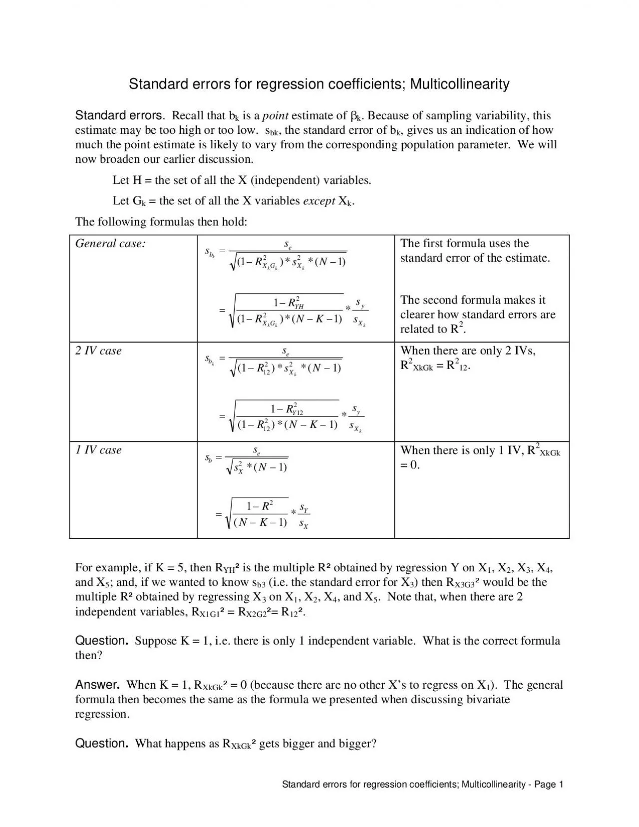
k General case kkkkkkkXyGXYHXGXebssKNRRNsRss11 ssRsNRRNKssbeXYyXkkk11111222122122 1 When there are only 2 IVs R 2 2 XkGk 0 For example if K 5 then R YH 5 is the multip ID: 937638

multicollinearity standard variables errors standard multicollinearity errors variables tolerance regression variable xkgk error bigger larger coefficients 146 variance correlated

Share:

Link:

Embed:

Download Presentation from below link

Download Pdf The PPT/PDF document "The following formulas then hold" is the property of its rightful owner. Permission is granted to download and print the materials on this web site for personal, non-commercial use only, and to display it on your personal computer provided you do not modify the materials and that you retain all copyright notices contained in the materials. By downloading content from our website, you accept the terms of this agreement.


Presentation Transcript

k . The following formulas then hold: General case: kkkkkkkXyGXYHXGXebssKNRRNsRss*)1(*)1( ssRsNRRNKssbeXYyXkkk()**()()*()*11111222122122 1 When there are only 2 IVs, R 2 2 XkGk = 0. For example, if K = 5, then R YH 5 is the multiple R5 obtained by regression Y on X 1 , X 2 , X 3 , X 4 , and X 5 ; and, if we wanted to know s b3 Answer. When K = 1, R XkGk 5 = 0 (because there are no other X’s to regress on X 1 ). The general formula then becomes the same as the formula we presented when discussing bivariate regression. Question. What happens as R XkGk 5 gets bigger and bigger? Standard errors for regression coefficients; Multicollinearity - Page 1 Answer. As R XkGk 5 gets bigger and bigger, the denominator in the above equations gets smaller and smaller, hence the standard errors get larger and larger. For example: If R 12 5 = 0, and nothing else changes, then, 209.478.4788.9*)17(*)01(84498.1*)1(*)1(1209.95.38008.4)19(*05.20*)01(08.4)1(**)1(1112122122212XyYXebssKNRRNsRss 171.461.5788.9*)17(*)01(84498.1*)1(*)1(1171.55.56608.4)19(*82.29*)01(08.4)1(**)1(2222122122212XyYXebssKNRRNsRss If R 12 5 = .25 and nothing else changes, then, 241.478.4788.9*)17(*)25.1(84498.1*)1(*)1(1241.71.28508.4)19(*05.20*)25.1(08.4)1(**)1(1112122122212XyYXebssKNRRNsRss 198.461.5788.9*)17(*)25.1(84498.1*)1(*)1(1198.935.42408.4)19(*82.29*)25.1(08.4)1(**)1(2222122122212XyYXebssKNRRNsRss Similarly, you can show that, if R 12 5 = .5, then s b1 = .295 and s b2 = .242. Question. Suppose R XkGk 5 is very large, say, close to 1. What happens then? Answer. If R Xk

Gk 5 = 1, then 1 - R XkGk 5 = 0, which means that the standard error becomes infinitely large. Ergo, the closer R XkGk 5 is to 1, the bigger the standard error gets. Put another way, the more correlated the X variables are with each other, the bigger the standard errors Standard errors for regression coefficients; Multicollinearity - Page 2 become, and the less likely it is that a coefficient will be statistically significant. This is known as the problem of multicollinearity. Intuitively, the reason this problem occurs is as follows: The more highly correlated independent variables are, the more difficult it is to determine how much variation in Y each X is responsible for. For example, if X 1 and X 2 are highly correlated (which means they are very similar to each other) it is difficult to determine whether X 1 is responsible for variation in Y, or whether X 2 is. As a result, the standard errors for both variables become very large. In our current example, if R 12 5 = .95, then s b1 = .933 and s b2 = .765. Note that, under these conditions, neither coefficient would be significant at the .05 level, even though their combined effects are statistically significant. Comments: 1. It is possible for all independent variables to have relatively small mutual correlations and yet to have some multicollinearity among three or more of them. The multiple correlation R XkGk can indicate this. 2. When multicollinearity occurs, the least-squares estimates are still unbiased and efficient. The problem is that the estimated standard errors of the coefficients tend to be infl

ated. That is, the standard error tends to be larger than it would be in the absence of multicollinearity because the estimates are very sensitive to changes in the sample observations or in the model specification. In other words, including or excluding a particular variable or certain observations may greatly change the estimated coefficients. 3. One way multicollinearity can occur is if you accidentally include the same variable twice, e.g. height in inches and height in feet. Another common error occurs when one of the X’s is computed from the other X’s (e.g. Family income = Wife’s income + Husband’s income), and the computed variable and the variables used to compute it are all included in the regression equation. Improper use of dummy variables (which we will discuss later) can also lead to perfect collinearity. These errors are all avoidable. However, other times, it just happens to be the case that the X variables are naturally highly correlated with each other. 4. Many computer programs for multiple regression help guard against multicollinearity by reporting a “tolerance” figure for each of the variables entering into a regression equation. This tolerance is simply the proportion of the variance for the variable in question that is not due to other X variables; that is, Tolerance X k = 1 - R XkGk 2 . A tolerance value close to 1 means you are very safe, whereas a value close to 0 shows that you run the risk of multicollinearity, and possibly no solution, by including this variable. Note, incidentally, that the tolerance appears in t

he denominator of the formulas for the standard errors. As the tolerance gets smaller and smaller (i.e. as multicollinearity increases) standard errors get bigger and bigger. Also useful is the Variance Inflation Factor (VIF), which is the reciprocal of the tolerance. This shows us how much the variances are inflated by multicollinearity, e.g. if the VIF is 1.44, multicollinearity is causing the variance of the estimate to be 1.44 times larger than it would be if the independent variables were uncorrelated (meaning that the standard error is 1.44 = 1.2 times larger). Standard errors for regression coefficients; Multicollinearity - Page 3 5. There is no simple means for dealing with multicollinearity (other than to avoid the sorts of common mistakes mentioned above.) Some possibilities: a. Exclude one of the X variables - although this might lead to specification error b. Find another indicator of the concept you are interested in, which is not collinear with the other X’s. c. Put constraints on the effects of variables, e.g. require that 2 or more variables have equal effects (or effects of equal magnitude but opposite direction.) For example, if years of education and years of job experience were highly correlated, you might compute a new variable which was equal to EDUC + JOBEXP, and use it instead. d. Collect a larger sample, since larger sample sizes reduce the problem of multicollinearity by reducing standard errors. e. In general, be aware of the possible occurrence of multicollinearity, and know how it might distort your parameter estimates and significa

nce tests. Here again is an expanded printout from SPSS that shows the tolerances and VIFs: Coefficientsa -7.097 3.626 -1.957 .067 -14.748 .554 1.933 .210 .884 .096 9.209 .000 1.490 2.376 .846 .913 .879 .989 1.012 .649 .172 .362 .096 3.772 .002 .286 1.013 .268 .675 .360 .989 1.012 (Constant) EDUC JOBEXP Model 1 B Std. Error UnstandardizedCoefficients Beta Std. Error StandardizedCoefficients t Sig. Lower Bound Upper Bound 95% Confidence Interval for B Zero-order Partial Part Correlations Tolerance VIF Collinearity Statistics Dependent Variable: INCOMEa. Standard errors for regression coefficients; Multicollinearity - Page 4 Another example. Let’s take another look at one of your homework problems. We will examine the tolerances and show how they are related to the standard errors. Mean Std Dev Variance Label XHWORK 3.968 2.913 8.484 TIME ON HOMEWORK PER WEEK XBBSESRW -.071 .686 .470 SES COMPOSITE SCALE SCORE ZHWORK 3.975 2.930 8.588 TIME ON HOMEWORK PER WEEK XTRKACAD .321 .467 .218 X IN ACADEMIC TRACK N of Cases = 9303 Equation Number 1 Dependent Variable.. XHWORK TIME ON HOMEWORK PER WEEK Multiple R .40928 R Square .16751 Standard Error 2.65806 Analysis of Variance DF Sum of Squares Mean Square Regression 3 13219.80246 4406.60082 Residual 9299 65699.89382 7.06526 F = 623.69935 Signif F = .0000 ------------------------------------- Variables in the Equation

------------------------------------- Variable B SE B 95% Confdnce Intrvl B Beta SE Beta Correl Part Cor XBBSESRW .320998 .042126 .238422 .403575 .075555 .009915 .179292 .072098 ZHWORK .263356 .009690 .244363 .282350 .264956 .009748 .325969 .257166 XTRKACAD 1.390122 .062694 1.267227 1.513017 .222876 .010052 .303288 .209795 (Constant) 2.496854 .049167 2.400475 2.593233 ---------- Variables in the Equation ---------- Variable Partial Tolerance VIF T Sig T XBBSESRW .078774 .910596 1.098 7.620 .0000 ZHWORK .271284 .942060 1.062 27.180 .0000 XTRKACAD .224088 .886058 1.129 22.173 .0000 (Constant) 50.783 .0000 To simplify the notation, let Y = XHWORK, X 1 = XBBSESRW, X 2 = ZHWORK, X 3 = XTRKACAD. The printout tells us N = 9303, SSE = 65699.89382, s e = 2.65806, R Y123 5 = .16751, s y = 2.913, s 1 = .686, s 2 = 2.930, s 3 = .467, Tolerance X 1 � = .910596 == R X1G1 5 = 1 - .910596 = .089404 Tolerance X 2 � = .942060 == R X2G2 5 = 1 - .942060 = .057940 Tolerance X 3 � = .886058 == R X3G3 5 = 1 - .886058 = .113942 The high tolerances and the big sample size strongly suggest that we need not be worried about multicollinearity in this problem. We will now compute the standard errors, using the information about the tolerances. Standard errors for regression coefficients; Multicollinearity - P