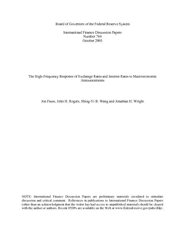
e Federal Reserve System Number 784 tes and Interest Rates to Macroeco - PDF document

e Federal Reserve System Number 784 tes and Interest Rates to Macroeconomic Announcements Jon Faust, John H. Rogers, Shing-Yi B. Wang and Jonathan H. Wright NOTE: International Finance Discussion Papers are preliminary materials circulated to stimulate discussion and critical comment. References in publications to International Finance Discussion Papers (other than an acknowledgment that the writer has had access to unpublished material) should be cleared with the author or authors. Recent IFDPs are available on the Web at www.federalreserve.gov/pubs/ifdp/. tes and Interest Rates to Macroeconomic Announcements Jon Faust, John H. Rogers, Shing-Yi B. Wang and Jonathan H. Wright : Many recent papers have studied movements in stock, bond, and currency prices over short windows of time around macro announcements. This paper adds to the announcement effects literature in two ways. First, we study the joint announcement effects across a broad range of assets--exchange rates and U.S. and foreign term structures. In order to evaluate whether the joint effects can be reconciled with conventional theory, we interpret the joint movements in light of uncovered interest rate parity or changes in risk premia. For several real macro announcements, we find that a stronger than expected release appreciates the dollar today, but that it must either (i) lower the relative risk premium for holding foreign currency rather than dollars, or (ii) imply considerable future expected dollar depreciation. The latter implies an overshooting behavior akin to that described by Dornbusch (1976). Second, we use a longer span of high frequency data than has been common in announcement work. A longer span of high frequency data contributes to the precision of our estimates and lity that the effects of macro surprises on asset prices have varied over time. We find evidence, for example, that PPI releases had a larger effect on Uncovered Interest Parity, Overshooting. International Finance Division, Board of Governors of the Federal Reserve System, Washington DC 20551. We are grateful to Alain Chaboud, Dale Henderson, participants in the 2003 NBER Summer Institute, and in the Association d’Econométrie Appliquée conference on Exchange Rates in Marseille for their helpful comments. The views in this paper are solely the responsibility of the authors and should not be interpreted as reflecting the views of the Board of Governors of the Federal Reserve System or of any person associated with the Federal Reserve System. The study of high frequency asset price movements has examined the relationships among the unexpected component of macroeconomic announcements and various asset returns. This paper contributes to the literature in two ways. First, we consider the joint effects of U.S. macro announcements on exchange rates and U.S. and foreign interest rates of various maturities. Most prior work has considered announcement effects on a single asset or asset class. The interpretations these papers place on measured effects generally have implications about how other asset prices should have reacted to the announcement. For example, Anderson, Bod Vega’s (2003a) (hereafter, ABDV) excellent study of the reaction of exchange rates to macro announcements finds that an announcement of U.S. retail sales that is greater than expected is associated with an appreciation of the dollar. This can be reconciled with conventional exchange rate theory, e.g., the monetary model, if the announcement portends higher-than-expected U.S. income, but this should also be reflected in a rise in U.S. interest rates. Studying the joint behavior of a broad range of asset returns allows us e market reaction to news. A second significant contribution of this paper is the use of a longer span of high frequency intradaily data than used in most other papers. Our sample includes data from 1987 to 2002, a period including 2 NBER recessions. Earlier work covers a much smaller time period. For example, ABDV’s sample is January 1992 to December 1998, a period in which the U.S. economy was always in an expansion phase. Fleming and Remolona (1997), in their study of bond returns, use a 1-year sample starting in mid- 1993. A longer sample period including a broader range of states of the economy should One reason for the short samples in earlier work is the limited availability of intradaily data. In estimating the effect of an announcement, it is desirable to measure the asset price changes in a narrow window around the time of the macro announcement. If we choose a window that is narrow enough, the information hitting the market during the window should be dominated by the macro announcement; thus, the events in the narrow window provide us an approximate natural experiment. Earlier work has shown that the average effect of announcements is completed very quickly, so that confining attention to a 20-minute window around the time of the announcement should be more daily changes, which include the effect of announcements and all other information hitting the market that day, leads to very imprecise estimates of the announcement effects. Nonetheless, many papers in the literature on announcement effects use daily data instead because long spans of intradaily data were not available until recently. It has proven very difficult to link asset price movements to macroeconomic fundamentals, but this is especially true for exchange rates (Meese and Rogoff (1983)). The systematic relationship between the surprise component of macroeconomic data releases and one-day exchange rate changes is weak and hard to detect (Hardouvelis The literature measuring the effects of macro announcements on asset prices at daily or intradaily frequency is vast and includesDornbusch (1980), Schwert (1981), Frenkel (1981), Edwards (1982), Cornell (1983), Pearce and Roley (1983), Frankel and Engel (1984), Ito and Roley (1987), Hardouvelis (1988), Cutler, Poterba and Summers (1989), McQueen and Roley (1993), Ederington and Lee (1993), Edison (1997), Fleming and Remolona (1997, 1999), Almeida, Goodhart and Payne (1998), Bollerslev, Cai and Song (2000), Clare and Courtney (2001), Kuttner (2001), Ehrmann and Fratzscher (2002), Gurkaynak, Sack and Swanson (2003) and Bernanke and Kuttner (2003). Some of these papers also document a systematic relationship between the announcements and the conditional variance of asset returns. (1988) and Edison (1997)). That is what makes the work of ABDV such a major contribution because it is able to pin down precisely estimated relations between macroeconomic surprises and exchange rate Fair (2003) is work closely related to this paper as it too considers high frequency intradaily data on a range of asset prices over a long period (1982 to 1999). He identifies occasions on which the five-minute change in stock prices, bond prices or exchange rates exceeded 0.75 percentage points, and then conducts newswire searches to identify an important event that occurred at that time. An event can be identified in many (though not all) cases, and this event is often a U.S. macroeconomic announcement. Fair lists these events and studies the correlations of changes in stock prices, bond prices and exchange rates around these events. This supports the view that U.S. macro announcements are important detime of the release. While Fair studies large events, we study the average effects of all announcements on changes in intereWe follow most of the macro announcements literature in focusing on the “surprise” component of the announcements. We study 10 announcements of U.S. indicators: CPI, PPI, Fed Funds target, GDP, unemployment rate, initial unemployment claims, housing starts, nonfarm payrolls, retail sales, and trade balance. For most releases, we measure the surprise component as the difference between the actual release and the Money Market Services (MMS) survey expectation. For the FOMC announcement about the target Fed Funds rate, we follow Kuttner (2001) in taking the expected change from the Fed Funds futures market. We discuss possible limitations of We obtain significant and quite precisely estimated effects for several macroeconomic releases on exchange rates and the term structure of U.S. and foreign interest rates. Stronger than expected real releases (e.g. nonfarm payrolls, retail sales, GDP) tend to appreciate the dollar and raise short and long-term interest rates in the U.S. and, to a lesser extent, overseas. Higher than expected inflation (CPI or PPI) is estimated to have little effect on the exchange rate, but to raise U.S. interest rates significantly. Tighter than expected monetary policy (i.e. a higher than expected target Fed Funds rate) is estimated to appreciate the dollar and to raise the term structure of U.S. interest rates. The effect on the 10-year U.S. interest rate is more precisely estimated and smaller than similar methodology, but using daily data. For the most part our point estimates for individual asset returns are quite similar to those of earlier work including ABDV (exchange rates, intradaily data), Ederington and Lee (1993) (exchange rates and U.S. interest rates, intradaily data), Fleming and Remolona (1997, 1999) (U.S. interest rates, intradaily data), Kuttner (2001) (U.S. interest rates, daily data) and Gurkaynak, Sack and Swanson (2003) (forward U.S. interest rates, daily data). Compared to work where only daily data has been used our inference is more precise and our results sometimes give a different picture. Our main goal of characterizing the joint movements of exchange rates and interest rate term structures presents a bit of a presentational challenge. Uncovered interest rate parity (UIP) is a convenient starting point. We know that UIP does not hold Gurkaynak, Sack and Swanson (2003) and Clare and Courtenay (2001) also consider the effect of UK macro announcements on UK interest rates. unconditionally: there seems to be a highly variable risk premium reflected in the joint movements of interest differentials and exchange rates. However, as an interpretational device we can assume that the announcements do not change the risk premium, in which case our estimated effects imply a trajectory of the exchange rate response to the macro news. If the trajectory is difficult to reconcile as an expected path of the exchange rate, one can reason about what must have happened to the risk premium. We investigate the implied risk premium behavior under the assumption that exchange rate expectations are consistent with a random walk model. For several real macro releases, such as nonfarm payrolls, we find that a stronger than expected release appreciates the dollar today, and that it either (i) lowers the risk premium for holding foreign rather than dollar-denominated assets, or (ii) implies future expected dollar depreciation in excess of the original jump. If one were to assert that a stronger-than-expected U.S. release the risk premium for holding foreign rather than dollar-denominated assets, our results imply that this could only be consistent with We find that higher-than-expected CPI and PPI releases also lower the foreign exchange risk premium and/or lead to significant long-run expectedAfter the first version of this paper was written, we became aware of independent concurrent related work by Anderson, Bollega (2003b). They consider the effect of the unexpected component of macroeconomic announcements on a wide range of international asset returns, including exchange rates, US and foreign stocks and bonds. The set of assets they consider is different from those in this paper. We do not include any stock returns, but, unlike include short term interest rate futures and so consider the effects of macro announcements on US and foreign interest rates ofturn motivates our analysis of the effect of announcements on the trajectory of expected future exchange rates and/or UIP risk premia. Our dataset also covers a longer time span. For example, our high frequency data on foreign interest rates goes from 1989 or earlier The plan for the remainder of this paper is as follows. Section 2 contains some theoretical discussion of the interpretation of a regression of high fron the unexpected component of macroeconomic announcements. Section 3 describes the data. Section 4 contains the basic regression results. Section 5 contains the analysis of the effects of surprises on expected future exchange rates and the UIP risk premium, that we can obtain only by studying the simultaneous responses of interest differentials and exchange rates to the data releases. Tests for parameter stability and models allowing for time-varying parameters are reporThe starting point of the announcements littt a small time window (say, 20 minutes) around a macro announcement, say for the CPI, and is the surprise component of the CPI announcement. Obviously, then measures the typical effect of the inflation surprise. The hope is that by focusing on a narrow time window, we get something like a natural experiment allowing us to learn the effects of a particular type of information. Although this approach is standard, there has been little the natural experiment In this section we present a simple framework within which to interpret this regression. While the assumptions are heroic, such assumptions are required to motivate the fixed-coefficient, linear model that a natural starting point for this sort of work. The bottom line is that the in the basic regression should be interpreted as a linear combination of the effects of every kind of fundamental shock in the economy where the weights have the interpretation as Kalman gain coefficients. We provide further interpretation below. Suppose there is a state variable f describing all variables in the economy that can be viewed as fixed in any 20 minute period. This includes the of productivity, non-auction market prices, and so on. Let f denote the public’s current view of this state. The equilibrium auction price of an asset, p , is a function of f and f (,)tttpff. Now linearize this system around (,) 001020ˆˆˆ(,)()()tttpffffffφφφ≈+−+− t f and 2ˆt f . Next time difference this equation over a 20 minute interval: Notice that if we are modeling the world as with a representative agent economy, for the purposes of an announcement effects paper, it must be an agent that does not know her own income or productivity. This is required because when data on income for a period ending several weeks earlier comes out, it affects markets. Similarly, inflation data for earlier periods affect the markets; thus, the agent does not know all past prices. The agents may know some elements of the state variable with certainty, but generally we allow all of them to be uncertain. '''112121ˆˆˆˆ()()()ttttttt ffffffφφφ ∆≈−+−=−where the second step comes from the fact that in the 20 minute window. Now take the conditional expectation of this expression conditional on f and dimensional information variable that is the only information arriving between and . Computing this expectation requires assumptions about how affects f . If all variables are covariance stationary and Gaussian, the effect of on f will be given by the standard Kalman updating so that 1s is the Kalman gain. Making the substitutions gives, 112[|,]tttttEpfsgsThus, we have that is a linear combination of price effects associated with a shock to public understanding of every state variable. These effects are collected in The weights, given by , indicate how much the particular announcement in question Suppose that is an inflation announcement and it comes in surprisingly low. One might deduce that productivity is greater than anticipated, that monetary policy will be looser in the future than previously thought, that the capital stock is bigger than previously thought, or that any other state variable is slightly different from what was previously thought (e.g., Alaskan oil reserves). We presumably think that it contains more information about, say, productivity, than about Alaskan oil reserves, implying that the Kalman gain associated with productivity is much larger than the Kalman gain on oil reserves. These gains then get multiplied by the effect of the state variable on prices to What this exercise demonstrates is that while we have a sort of natural experiment, it is not a simple one. Interpreting the slope coefficient involves telling stories about both how a given shock affects views of the state variables but also about how those state variables affect the economy. This analysis differs from some implicit analysis in other papers. For example, some early papers reasoned from the fact that because income and other state variables are fixed within the window, the movement in the shock could not be due to revisions in income. We think this is incorrect: it can be due revisions in the agent's view of income, productivity or the capital stock. Some analyses implicitly proceed as if we know that certain of the Kalman gain coefficients are large and that others are trivially small. Without such an assumption, there is no clear interpretation of any of the announcements. For example, the model Frankel and Engel (1984) use to illustrate exchange rate jumps in response to money supply announcements is based on the assumption that the money announcements shed no light on income and are informative only about future Fed Our approach makes clear that the linear, fixed coefficient approach rests on strong assumptions and motivates us to consider time variation in the effects of macro announcements on asset prices in section 6 below. With our long sample of high frequency data, spanning two recessions, we can shed light on such questions that we could not hope to answer with adequate precision using shorter samples. To take a specific case that may have been of relevance in the 1990s, if inflation is perceived to be evidence of weak demand, then agents might expect monetary policy to be loosened, causing interest rates to fall and the dollar to depreciate. But, if the unexpectedly low inflation is perceived to be evidence of productivity growth, then in some models U.S. interest rates rise and the dollar appreciates.We consider the effects on exchange rates and interest rates of 10 macroeconomic announcements, plus the FOMC day release of the decision about the target Federal Funds rate, as listed in Table 1. Nine of the announcements occur at 8:30am Eastern time; the target Fed Funds rate is released at 2:15pm Eastern time. The timing of the 8:30am macroeconomic announcements is extremely precise, while the Fed’s decision about the target Fed Funds rate has been announced on the FOMC day within a couple of minutes of 2:15pm since March 1995. For the 8:30 announcements, we measure the expected announcement using the median survey expectation from Money Market Services. The data come from the MMS survey of money managers taken the Friday before the release of the data. These survey See Glick and Rogoff (1995) and Erceg, Guerrieri and Gust (2002) for more discussion of the impact of productivity growth on real exchange rates and the trade balance. The latter paper argues that agents initially viewed the productivity acceleration in the U.S. in the 1990s as being transitory, but then came to believe that it represented a break in the trend growth rate of productivity. They back this up with survey evidence. In a dynamic general equilibrium model, they show that this can account for much of the deterioration of the U.S. trade balance, and the real appreciation of the dollar. Many other countries, including Germany, do not release macroeconomic data at precise scheduled times. From February 1994 to March 1995, the FOMC decision was explicitly announced, but at varying times. Prior to February 1994 it was not explicitly announced at all, but rather had to be inferred from the Desk’s subsequent activity. data have been widely used and the properties have been much studied. They are generally found to possess reasonable properties as expectations series, as they are unbiased, pass simple forecast rationality tests, and outperform naive time series forecasts (see, for example, Balduzzi, Elton and Green (2001)). We measure the surprise component of the announcement as the actual data release less the MMS survey expectation. Our sample runs from January 1987 through December 2002, though for some of the announcements, the MMS data do not go all the way back to the start of our sample: in these cases we just use the data as far back as possible. Data availability and the units in which the data are recorded are noted in Table 1. We handle the target Federal Funds rate differently. Although MMS records survey expectations for the target Fed Funds rate, we instead measure the surprise component of the Fed’s decision from intradaily changes in Federal Funds futures. We do this by the following algorithm, which is an adaptation of that proposed by Kuttner (2001) for daily data. If the FOMC meeting is on or before the 22nd of the month, take the change in the current month Fed Funds futures price from 2:10 to 2:30 and scale the change by the ratio of the total number of days in the month to the total number of days left in the month, to obtain the surprise change in the target Fed Funds rate. This scaling is necessary because the contract settles to the average interest rate in the month. If the FOMC meeting is on or after the 23rd of the month, we measure the surprise change in the target Fed Funds rate as the change in the next month Fed Funds futures price from 2:10 to 2:30. The Fed Funds futures give a better measure of expectations of target Fed The reason for using the next month futures price change rather than the scaled change in the current month futures price change is because the data are recorded only to the nearest basis point (half basis point since 1995), so our measured surprise change has rounding error that would be exacerbated by the scaling. Funds rate changes than MMS survey expectations in the sense that in a regression of the actual realized target Fed Funds rate on the forecasts from the futures market and the res rate is not significantly different from one, while the coefficient on the survey forecast is not significantly different from zero. Our exchange rate data consist of the 5-minute exchange rate returns for dollar exchange rates versus the DM/euro and pound, covering the entire calendar years 1987 to 2002 inclusive, from Olsen and Associates. To construct these darecord all Reuters quotes, average the bid and ask, and then linearly interpolate the resulting series to get prices at exactly the required times. From these data, we construct exchange rate returns over 20-minute windows starting 5 minutes before the data release, and ending 15 minutes after the data release. For an 8:30 data release, we construct exchange rate returns from 8:25 to 8:45. For an FOMC release, we construct exchange rate returns from 2:10 to 2:30. Throughout this paper, we construct exchange rates as dollars per unit foreign currency, so that a positive exchange rate return represents an appreciation of the foreign rate returns are continuously compounded, and multiplied by 10,000, so they can be interpreted as (approximately) the exchange rate This consists of the HFDF2000 dataset covering the years 1987 to 1998, with an extension through the end of 2002, also purchased from Olsen. We could simply use exchange rate returns from the moment of the announcement until 5 minutes later, but do not for two reasons. First, although ABDV find that the response of exchange rates to macroeconomic announcements is fast, for some announcement-currency pairs they find that the full effect on the conditional mean takes a little more than 5 minutes. Second, since the data are based on linearly interpolated quotes, the exchange rate data for 8:30 may incorporate a quote that came after an 8:30 release. Taking exchange rate returns from 8:25 to 8:45 effectively circumvents this problem. Interest Rate DataOur interest rate data consist of tick-by-tick transactions prices for Federal Funds futures, 3-month Eurodollar, euromark/euribor and sterling libor futures contracts, 10 year Treasury bond futures, and 10 year UK and German bond futures going back to the late 1980s. The exact dates for which we have data on each of these instruments are shown in Table 2. We obtained U.S. futures data from Genesis, and foreign futures data from the Futures Exchange (LIFFE) and the EUREX Exchange in Federal funds futures trade at the Chicago Board of Trade (CBOT). There is a contract for every month. The settlement price for each contract is the average effective Fed Funds rate for that month. Contracts trade for each of about the next 8 months, but only the first few contracts are liquid. Eurodollar contracts trade at the Chicago Mercantile Exchange (CME). There is a contract for settlement in March, June, September and December of each year. The settlement price for each contract is simply the 3-month eurodollar deposit rate on the settlement day. Ten year Treasury bond futures trade on CBOT. Again, there is a contract for settlement in March, June, September and December of each year. Euromark/euribor and sterling libor contracts trade on LIFFE. They are similar to eurodollar contracts, except that they settle to mark/euro and sterling 3-month interest rates. The 10 year UK and German bond futures also trade on LIFFE and are similar to 10 year Treasury bond futures. Since 1999, liquidity in German bond futures has switched to EUREX and we use EUREX data for German bond futures instead. Trading in interest rate futures at 7:20am Central Time, so all of the futures are trading at 8:30am Eastern time. All of the US contracts are trading at 2:15pm Eastern Time, but LIFFE and EUREX are closed at this time. From these data, we construct zero-coupon rates at maturities 3 months and 1-10 years at 8:25am and 8:45 am, for the US, the UK and Germany, using the method described in the appendix. We also construct zero-coupon rates at these maturities at 2:10 and 2:30 for the US alone in the same way. Hence we construct changes in zero-coupon interest rates at these 11 different maturities in 20-minute windows starting 5 minutes before the data release, and ethe data release. For each of the 10 macroeconomic releases, we run regressions of exchange rate returns and interest rate changes over 20-minute windows around the time of the macroeconomic data release, , on the surprise component of the data release, s . As noted above, the ttt (1) While heteroskedasticity is not necessarily a first-order issue in these regressions, we use t White standard errors. We note that the regressor could well be affected by measurement error, biasing the estimated coefficient towards zero. Indeed this concern motivates us to measure the surprise component of the target Fed Funds rate Results including a constant are not substantially different, and are available from the authors on request. The regression could be specified to allow positive and negative surprises to have asymmetric effects. The results for these regressions are available from the authors on request, but are not shown because there is only limited evidence of such asymmetry. from intradaily futures rates rather than from MMS surveys, so as to avoid, or at least minimize, measurement error in this surprise. In Table 3, we report the point estimates and the (uncentered) regression R-squared for the regression of each exchange rate return on each macroeconomic surprise. These regressions are run only over the 20-minute windows around the time of the macroeconomic announcement: for the announcements that are made monthly this means that there is one observation per month. The interpretation of the rethe fraction of the variance of the exchange rate in that 20-minute window that is explained by the announcement, which is of course not at all the same thing as the rate variance that is explained by the announcement. We have very similar qualitative results to ABDV, although our sample period is substantially longer than theirs. The announcements are such that positive surprises growth or higher-than-expected inflation. For the unemployment rate and initial jobless claimscyclical indicators, we flip the sign of the surprise so that positive surprises reflect stronger-than-expected growth for these indicators as well. The point estimates in Table 3 generally indicate that stronger-than-expected announcements lead to negative exchange rate returns, i.e. dollar appreciation. The effect is statistically significant for some, though not all, announcement-currency pairs. The elements of Table 3 can be interpreted as the effect of a one unit surprise in the macroeconomic release on the exchange value of the dollar, Note however that ABDV define exchange rates as foreign currency per dollar, whereas we define exchange rates as dollars per foreign currency, so their coefficient estimates are mostly positive. Also note that ABDV normalize the macroeconomic surprises to have unit standard deviation, which we do not. in basis points. The point estimates are quite small -- for example if GDP comes out one percentage point above expectations (quarter-over-quarter, at an annualized rate), the estimated effect is to apprher currencies by only about 10 basis points. Some announcements are more systematically related to exchange rates than others. GDP, initial unemployment claims, nonfarm payrolls, retail sales, the trade balance, unemployment and the FOMC decision on the target Fed Funds rate are all significant at the 1% level for both currencies, with a surprise monetary policy easing being associated with dollar depreciation. The R-squared (over the 20-minutes around announcements) is over 20% for some announcement-currency pairs. Although such an association is weak, it is still a triumph by the dismal standards of modeling the and macroeconomic fundamentals. Results for Interest Rate ChangesWe regress the changes in interest rates of different horizons on each macro surprise and plot the coefficients against the horizon of the interest rate in Figures 1 and 2. These figures represent the effects of a one unit surprise in the U.S. macro announcement on the term structure of U.S. and foreign interest rates. Stronger-than-expected releases tend to raise U.S. interest rates, including long-term interest rates, and the effects are in many cases statistically significant. Stronger-than-expected U.S. releases also tend to raise foreign interest rates, although by a smaller amount. In the United States, there are three releases of GDP during our sample period (aside from annual and benchmark revisions). The advance release comes out about 1 month after the end of the quarter to which it refers. The next two releases (called preliminary and final) are revisions that come out about 2 and 3 months after the end of the quarter, respectively. In our data analysis we are using just the advance release. The effect of a shock to the Fed Funds rate on the term structure of interest rates is of special interest. A great many papers have considered estimation of the effect of a change in the Fed Funds rate on the term structure of interest rates including Cook and Hahn (1989), Radecki and Reinhart (1994), Roley and Sellon (1995) and Kuttner (2001). The conventional view of the monetary policy transmission mechanism is that a shock to the Fed Funds rate affects consumption and investment demand through its effect on long-term interest rates. If long-term interest rates are insensitive to shocks to the Fed Funds rate then monetary policy is either ineffective, or must work through other channels (Barth and Ramey (1991) Kuttner (2001) regresses one-day changes in the U.S. yield curve on the unexpected component of the change in the Federal Funds rate, as measured from daily closing prices in the Fed Funds futures market. Our regression of the U.S. term structure on the unexpected component of the change in the Federal Funds rate is similar to that of Kuttner, but we use intradaily data both to measure the monetary policy surprise, and to measure the effect of the surprise on other interest rates. Our results are not inconsistent with those of Kuttner, but point to smaller and more precisely estimated effects of the monetary policy shock on long-term interest rates. Kuttner estimated that a 100 basis point unexpected tightening of monetary policy raises 10-year yields by 31.5 basis points, with a standard error of 10.2 basis points. When Kuttner includes FOMC days on which no change in rates actually occurred, the estimate falls to 22.0 basis points, with a standard error of 9.2 basis points. Our estimate for the effect of a 100 basis point unexpected tightening in the Fed Funds rate on the 10-year U.S. interest rate is 13.3 basis points, with a standard error of 6.2 basis points. These very small estimates of the effects of monetary policy shocks on long-term interest rates are very close to those obtained by Roley and Sellon (1995) and Radecki and Reinhart In comparing our results with those of Kuttner (2001), note that we run our regression only over FOMC days since March 1995. It is only for these announcements that the release came in a scheduled announcement at 2:15. Demiralp and Jorda (2003), using daily data, report some evidence that the effect of monetary policy shocks on long-term interest rates was higher before 1994 than subsequently, and is higher for intermeeting moves than for target Fed Are Announcement Days Different? Our primary focus in this paper is on the effects of announcements on the conditional mean of asset prices, not their conditional variance. But for our method in this paper to be reasonable, it should be that asset price changes are more variable during the announcement window than in otherwise comparable windows. In Table 4, we report the standard deviation of intradaily exchange rate and interest rate changes over the 20 minutes bracketing each of the 10 macroeconomic announcements, relative to the intradaily exchange rate or interest rate change over the same 20 minutes on days when there is no macroeconomic announcement at all in that time interval. For example, the column of the table labeled CPI reports the standard deviation of exchange rate and interest rate changes between 8:25am and 8:45am on days when there is a CPI release divided by the standard deviation of the analogous changes between 8:25am and 8:45am on days when there is no 8:30am macro release at all. The Fed Funds column reports the standard deviation of exchange rate and interest rate changes between 2:10pm and 2:30pm on FOMC days divided by the standard deviation of the analogous change at that time on non-FOMC days. Most of the elements of this table are greater than 1, indicating that exchange rates and interest rates are indeed more volatile around announcements than at the same time on non-announcement days. Releases of CPI, PPI, GDP, retail sales, the employment report and the target Fed Funds rate are all associated with substantially elevated volatility. We next turn to studying the simultaneous effect of macroeconomic announcements on exchange rates and interest rates. Consider the UIP relationship tkttktk eeii ) is the domestic (foreign) k-period interest rate, is the log of the nominal exchange rate in home currency units per foreign, and denotes the time-t expectation. Under rational expectations and risk-neutrality, a testable proposition is that tktkktktkteeii =+−+ should be equal to unity (and equal to zero). This is nearly uniformly rejected in the data, however, as is typically found to be negative, i.e., the currency with the higher interest rate typically (Engel, 1996). A familiar interpretation of the empirical failure of UIP posits the existence of a time-varying risk premium, such ,,,tkttktktkEeeii −=−+ (2) This risk premium is the expected excess return that agents require to hold foreign rather than dollar-denominated bonds. Equation (2) is simply a definition of the risk premium, which one may prefer to think of as the expected UIP deviation. Of course, UIP does not hold, and the deviations from UIP, Consider the algebraic identity obtained from taking the difference in equation (2) from before to after the announcement ,,,tkttktktkEeeii =+−+ (3) where the hat denotes the change in the variable from just before to just after the announcement. We can measure and directly. From this we know tktk , but not each component separately. If we make an assumption about either term, we can measure the other. We first assume that the macro announcements do not affect the risk premium ). In this case, tkttktkEeeii and we can immediately compute the effect of the announcement on the expected future exchange rate as the effect of the announcement on ttktkeii . We relate this in turn to the macro surprise by estimating the regression, ttktkktteiis −=+ (4) Thus, under the assumption that the risk premium is unaffected by the macro announcement, the expected future exchange rate response to a one unit announcement surprise at horizon is simply the coefficient In Figures 3 and 4 we plot the coefficients obtained from estimating equation (4) separately for = 0, 3 months and 1-10 years (at horizon 0, equation (4) reduces to equation (1) and the conditional UIP assumption is not required). These plots show the effect of a unit macro surprise on the expected future trajectory of exchange rates. Also shown are 90% confidence intervals, obtained from heteroskedasticity-robust standard errors in (4). For the real announcements, the general pattern is that a stronger than expected announcement appreciates the dollar. But, assuming that the announcement does nothing to the UIP risk premium, this appreciation is not expected to last, and typically is expected to be more than reversed. For example, a release of higher-than-expected nonfarm payrolls data causes a significant appreciation of the dollar today, but causes an expected depreciation in 10 years time. This trajectory of exchange rates is akin to the for shocks to the money supply. For the price indexes (CPI and PPI), assuming that the announcement does nothing to the UIP risk premium, the projection coefficients imply that a higher than expected inflation number leads to significant expected future dollar depreciation. The assumption that the risk premium is not affected by the data release is questionable. A second exercise that helps us to reason about the risk premium begins with assuming that exchange rate expectations are given by the random walk model at all points in time. Under this assumption, the effect of the announcement on is given by the change in the interest differential tktk . Thus, we can estimate the effect of announcements on the risk premium by regressing tktk The effect of the U.S. macro announcement on the risk premium under the random walk assumption is plotted against the horizon in Figures 5 and 6; the risk premium is expressed at annualized rate. Generally stronger-than-expected U.S. releases lead to significant and large declines in the risk premium. Jointly, the two exercises lay out two possibilities. Either stronger-than-expected real macro news leads to expectations of dollar depreciation in the long-run, or lead to declines in the required risk compensation for holding foreign rather than dollar denominated assets. While we do not have good models for explaining empirically observed risk premia, one might have supposed that good macro news in the U.S. would raise the relative risk in owning foreign assets. If this were the case, even steeper dollar lied in the long-run. The idea that a stronger-than-expected real U.S. data release that leads initially to dollar appreciation would then lead to long-term depreciation can be reconciled with theory. The macro news could indicate higher relative real rates in the short-term (say, due to a policy response) but higher inflation and nominal rates in the long-term. This is the story laid out by Gurkaynak, Sack and Swanson (2003) to account for their results on the U.S. term structure. Note however that Alvarez, Atkeson and Kehoe (1999, 2003) propose a general equilibrium model in which agents have to pay a fixed cost to exchange money for assets. In this model, a positive shock to U.S. money growth raises the U.S. inflation rate, induces more agents to pay the fixed cost and participate in asset markets, and thereby lowers the foreign exchange risk premium. With our dataset covering the years 1987 to 2002, which spans two NBER recessions, we can address questions that we could not hope to answer with adequate precision using shorter samples. In particular, we can study time variation in the effect of macroeconomic releases on exchange rates and interest rates. The effect of macro surprises could vary across the business cycle or other economic conditions (see, for example, Boyd, Jagannathan and Hu (2001), Orphanides (1992), David (1997), Veronesi (1999), David and Veronesi (2001) and Ehrmann and Fratzscher (2002)). Tests of the null of parameter constancy in equation (1), using the structural stability test statistic proposed by Nyblom (1989), and using the sup-F statistic (the maximum value of the Chow statistic over all possible break dates) are reported in Tables 5 and 6, respectively. For most asset-announcement pairs, the hypothesis of parameter constancy is not rejected. Time-variation in the effect of announcements on exchange rates and interest rates does not generally seem to be a first order issue. There are however some notable exceptions. The hypothesis of parameter constancy is rejected in the regression of exchange rate returns on trade balance surprises. The hypothesis of parameter constancy is rejected in the regression of U.S. interest rates on PPI, CPI and nonfarm The null limiting distribution of this statistic was provided by Andrews (1993). We exclude break dates in the first and last 15% of the sample (see Andrews (1993)). Rose (1984) and Irwin (1989) are two early papers examining this relationship. Given that the effects of certain pieces of macroeconomic news seem to vary over time, we next turn to modeling the relationship between macroeconomic surprises and exchange rates in models that allow for parameter instability. The Random Coefficient Regression ModelA widely used statistical model that allows for time-variation in regression parameters is the random coefficient model of Rosenberg (1972), Cooley and Prescott (1973), and Watson and Engle (1983). In the context of the regression of a change in interest rates or exchange rate returns on announcement surprises, the model can be written as ttttttt (5) Under an assumption of normality in the errors, the parameters of the model in equation (5) can be estimated by maximum-likelihood. Taking the maximum likelihood estimates as given, we can do infere conditional on the entire sample, using the Kalman smoother, which also provides associated standard errors. The smoothed coefficient estimates reflect our beliefs at the end of the sample period about what the responsiveness of the asset price to macroeconomic surprises was, at each point in time. We applied this model to the effect of nonfarm payroll, PPI and trade balance surprises on exchange rates and interest rates. We picked these three announcements, because there was some evidence of parameter instability in each of their effects. The smoothed estimates of the effects of a surprise in nonfarm payrolls, PPI and the trade See Harvey (1991). We initialize the Kalman filter with a diffuse prior. balance are shown in Figures 7, 8 and 9, respectively. Results for CPI (not shown) are quite similar to those for PPI. In Figure 7, we see that the sensitivity of 3-month U.S. interest rates to nonfarm payrolls releases has declined since the early 1990s. The sensitivity of the exchange rate response to nonfarm payrolls surprises peaked in the early 1990s and has declined since In Figure 8, we see that the sensitivity of interest rates to PPI announcements was high in the early years of the sample, but then declined and is different from zero, for interest rates of any maturity. This could reflect the interpretation of PPI news as conveying news about stronger-than-expected productivity growth, rather than demand strength, later in the sample. In Figure 9, we see that the sensitivity of the exchange rate to news about the trade balance was very high in the early years of the sample, but it has subsequently waned and is no longer significantly different from zero. Trade balance releases never had much effect on short term U.S. interest rates. However, a lower than expected trade deficit was estimated to lead to a reduction in 10-year U.S. interest rates in the early part of the sample, but this effect has since waned too. Indeed, the decline in the effect of trade balance surprises on 10-year yields mirrors the decline in its effect on the exchange value of the dollar. An interpretation of this time variation in the effect of trade balance data is that in the 1980s and early 1990s, investors worried about the sustainability of the current account. Higher than expected trade deficits would be interpreted as a sign that the current account deficit is unsustainable, leading to dollar depreciation. It could also lead to an increase in yields on 10-year government bonds as the U.S. would have to offer more attractive yields to continue to get fore But, perhaps, beginning in the mid 1990s, investors started to think of the trade deficit as reflecting a positive country-specific productivity shock, as U.S. residents seek to smooth their consumption by borrowing from abroad in anticipation of higher future income. Arguably, investors paid little attention to the possibility of a break in the trend growth rate of productivity until the mid-1990s. At that point, however, they may well have begun to take seriously the idea of a break, and hence became more prone to interpret macroeconomic data surprises as conveying news about productivity. If so, higher than expected trade deficits would be interpreted as positive productivity shocks appreciation, by the Balassa-Samuelson effect. Existing work on high frequency movements in asset prices has documented the relationship between macroeconomic announcements and asset returns around those announcements. The literature has typically focused on a single asset or asset class, in isolation of other markets which theory predicts should move simultaneously. Much of this work has used a relatively short sample period and/or calculated asset returns over In this paper we contribute to this literature by studying the joint behavior of exchange rates and zero coupon interest rates using a long span of high frequency data. We interpret the joint behavior of exchange rates and interest rates in the context of uncovered interest rate parity, thereby obtaining evidence on the interaction between UIP risk premia and expected exchange rate dynamics, conditional on (U.S.) macro announcements. Our work is not a test of UIP; rather, it characterizes combinations of risk premium and expected exchange rate dynamics in response to macro news that are consistent with the data. We find that for several real U.S. macro announcements better than expected news appreciates the dollar today, consistent with existing evidence. From the responses of U.S. and foreign interest rate term structures, we are also able to infer that such releases either lower the risk premium for holding foreign currency or imply future expected dollar depreciation that exceeds the original appreciation. While we do not have good models for explaining empirically observed risk premia, one might have supposed that good macro news in the U.S. would raise the relative risk in foreign assets. If it is implausible that stronger than expected U.S. news lowers the risk premium on foreign assets, then this could only be consistent with an even steeper path of expected dollar depreciation following the initial appreciation. This would of course be inconsistent with a random walk formulation of expected exchange rate movements. Finally, there is some evidence of parameter instability for some announcements. Estimating models that allow for time varying parameters, we find that the effect of price surprises on interest rates has declined over our sample period and that the effect of trade balance surprises on exchange rates has also declined. We also find some evidence for time variation in the effects of ucted zero-coupon yield curves from interest rate and government bond futures. We have high frequency data on the first four eurodollar, euromark/euribor and sterling libor futures contracts. These contracts are all cash-settled to 3-month interest rates on the settlement day. By combining the prices on these short-term interest rate contracts, we obtain 3-month We also have high frequency data on the prices of 10-year bond futures in the US, the UK and Germany. These futures are nominally on 10-year bonds with a specific coupon rate (e.g. presently 6% for the CBOT 10-year contract). More precisely, the futures contract is fulfilled by the party on the short side of the contract delivering any bond in a particular maturity range (e.g. presently 6.5 to 10 years for the CBOT 10-year contract) to the party on the long side of the contract at a price equal to the futures price multiplied by a conversion factor to adjust the actual coupon rate of the delivered bond to the nominal coupon rate of the futures contract (plus an adjustment for accrued interest). The party on the short side will choose the bond that is cheapest to deliver, comparing the price that she will receive for the bond relative to the value of the bond in the spot market at the time of settlement. If interest rates are below the nominal coupon rate of the the short side will typically choose to deliver a bond at the short end of the maturity range, and vice-versa. From CBOT, LIFFE and EUREX, we obtained data on the bond that was delivered for each futures contract (or the most commonly delivered bond in cases where multiple bonds were delivered). We make the assumption that agents knew that this bond would be delivered, and treat the price of the front bond futures contract, multiplied by the conversion factor, as though it were the spot price of the bond that was in fsettlement of the contract. There exist bond contracts for settlement in March, June, September and December of each year. Contracts trade for each of about the next 4 settlement dates, but only the first one or two contracts are liquid. Moreover, liquidity in a bond futures contract decays sharply during the settlement month. We therefore define the “front” bond futures contract to be the June contract in March, April and May alone, and similarly for the Notice that we treat the high frequency futures-based interest rates and bond prices (with a near settlement date) as though they are the underlying spot interest rates and bond prices. Trading in short-term interest rate and bond futures markets is extremely liquid: liquidity in the bond futures market is far greater than in the market for any one specific bond issue. The futures and spot instruments are very close substitutes. Besides, our cross-country long span of high frequency data is on futures instruments, not spot instruments. In this sense we do not have a choice. We fitted the following standard zero-coupon yield curve, used by Diebold and Li 123()()()tttλτλτ τβββλτλτ=++− denotes the continuously-compounded zero-coupon yield of a bond with maturity and where . The parameters t and are time-varying and may be thought of as level, slope and curvature, respectively. This zero curve implies a price for the delivered bond in the bond futures contract. If the coupon payments on the delivered bond are at times ,,... (semiannual for the US and UK, annual for Germany), each coupon payment is of an amount c, and the bond is redeemed p , on the date of the final coupon, then the price of the delivered bond should be pcepe =Σ+We solve for these parameters t and at each point in time by simply requiring matches the 3 month and 1 year zero-coupon rates obtained from the short-term interest rate futures contracts and that () matches the price of the bond futures contract (multiplied by the conversion factor for the delivered bond). In this way, we have a set of three equations in three unknowns and can get an exact fit for the parameters of the zero-coupon yield curve. We then simply compute the zero-coupon yield at the required maturities. The structure of interest rate and bond futures contracts for the US, UK and Germany is remarkably similar, and so exactly the same methodology can be used for the US, UK and German zero-coupon yield curves. It is to preserve cross-country comparability of methodology that we do not use prices of CBOT 5 year Treasury bond futures, even though we have these data too. There is no comparable futures contract for y of such a contract for German bonds This procedure for obtaining high frequency observations on a zero-coupon yield curve is far from ideal. It effectively obtains the yield curve from just 3 points, which is fewer than is used in standard yield curve analysis (though can still identify level, slope and curvature). It treats the interest rate and bond futures prices as though they were spot prices. The party on the short side of the bond futures contract in fact has the option of choosing which bond to deliver, and the futures price incorporates the value of this optionality. By assuming that the parties to the futures contract knew ahead of time which bond would in fact be delivered, we are neglecting this option value. Also, our zero-coupon yield curve is neither a pure eurodollar nor a pure Treasury yield curve. Treasury and eurodollar interest rates are different because the latter incorporate some credit risk. The spread between Treasury and eurodollar rates, known as the TED spread, reflects the premium for this credit risk, and is typically about 20 basis points or less, but can be higher at times of market stress. We are quite aware of these shortcomings. However, our object of ultimate interest is not the zero-coupon yield curves themselves, but rather the in zero-coupon rates from just before to just after a macro announcement. Many of these issues we cite above are likely to have about the same effect on the yield curve before and after the macro announcement, and so will difference out. For example, unless the macro announcement has a large effect on the TED spread, the inappropriate mixing of Treasury and eurodollar prices should approximately difference out. It likewise seems plausible to us to assume that the value of the delivery option held by the party on the short side of a bond futures contract should approximately difference out. References Almeida, A., C. Goodhart and R. Payne (1998): The Effects of Macroeconomic News on ge Rate Behavior, Journal of Financial and Quantitative Alvarez, F., A. Atkeson and P. Kehoe (1999): Volatile Exchange Rates and the Forward Premium Anomaly: A Segmented Asset Market View, mimeo. Alvarez, F., A. Atkeson and P. Kehoe (2003): Time-Varying Risk, Interest Rates and Exchange Rates in General Equilibrium, Federal Reserve Bank of Minneapolis Andersen, T.G., T. Bollerslev, F.X. Diebold and C. Vega (2003a): Micro Effects of Macro Announcements: Real-Time Price Discovery in Foreign Exchange, Andersen, T.G., T. Bollerslev, F.X. Diebold and C. Vega (2003b): Real-Time Price ign Exchange Markets, mimeo. Andrews, D.W.K. (1993): Tests for Parameter Instability and Structural Change with Balduzzi, P., E.J. Elton and T.C. Green (2001): Economic News and Bond Prices: Evidence from the U.S. Treasury Market, Journal of Financial and Quantitative Barth, M.J. III and V.A. Ramey (2001): The Cost Channel of Monetary Transmission, NBER Macroeconomics Annual, MIT Press. Bernanke, B.S. and M. Gertler (1995): Inside the Black Box: The Credit Channel of Monetary Policy Transmission, Bernanke, B.S. and K.N. Kuttner (2003): What Explains the Stock Market’s Reaction to Federal Reserve Policy?, mimeo. Bollerslev, T., J. Cai and F.M. Song (2000): Intraday Periodicity, Long Memory Volatility, and Macroeconomic Announcement Effects in the U.S. Treasury Bond Journal of Empirical FinanceBoyd, J.H., R. Jagannathan and J. Hu (2001): The Stock Market’s Reaction to Unemployment News: Why Bad News is Usually Good for Stocks, NBER Clare, A. and R. Courtenay (2001): Assessing the Impact of Macroeconomic News Announcements on Securities Prices Under Different Monetary Policy Regimes, Bank of England Working Paper. Cook, T. and T. Hahn (1989): The Effect of Changes in the Federal Funds Target on Market Interest Rates in the 1970s, Journal of Monetary Economics, 24, pp.331-Cooley, T.F. and E.C. Prescott (1973): An Adaptive Regression ModelCornell, B. (1983): The Money Supply Announcements Puzzle: Review and Interpretation, American Economic Review, 73. pp.644-657. Cutler, D.M., J.M. Poterba and L.H. Summers (1989): What Moves Stock Prices?, Journal of Portfolio ManagementDavid, A. (1997): Fluctuating Confidence in Stock Markets: Implications for Returns and David, A. and P. Veronesi (2001): Inflation and Earnings Uncertainty and the Volatility of Asset Prices, mimeo. Demiralp, S. and O. Jorda (2003): The Response of Term Rates to Fed Announcements, , forthcoming. Diebold, F.X. and C. Li (2002): Forecasting the Term Structure of Government Bond Yields, Penn Institute for Economic Research Working Paper 02/026. Dornbusch, R. (1976): Expectations and Exchange Rate Dynamics, Journal of Political Dornbusch, R. (1980): Exchange Rate Economics: Where do We Stand?, Papers on Economic ActivityEderington, L. and J.H. Lee (1993): How Markets Process Information: News Releases Edison, H. (1997): The Reaction of Exchange Rates and Interest Rates to News Releases, s, Expectations and New Information, Journal of Monetary EconomicsEhrmann, M. and M. Fratzscher (2002): Interdependence Between the Euro Area and the US: What Role for EMU?, mimeo, European Central Bank. Engel, C. (1996): The Forward Discount Anomaly and the Risk Premium: A Survey of Recent Evidence, Erceg, C.J., L. Guerrieri and C. Gust (2002): Productivity Growth and the Trade Balance in the 1990s: The Role of Evolving Perceptions, mimeo. Fair, R. (2003): Shock Effects on Stocks, Bonds and Exchange Rates, Journal of Faust, J. and J.H. Rogers (2003): Monetary Policy’s Role in Exchange Rate Behavior, Journal of Monetary Economics, forthcoming. Fleming, M.J. and E.M. Remolona (1997): What Moves the Bond Market?, Fleming, M.J. and E.M. Remolona (1999): Price Formation and Liquidity in the U.S. Treasury Market: The Response to Public Information, Journal of Finance, 54, Frankel, J.A. and C. Engel (1984): Why Interest Rates React to Money Announcements: An Explanation from the Foreign Exchange Market, EconomicsFrenkel, J.A. (1981): Flexible Exchange Rates, Prices and the Role of ‘News’: Lessons from the 1970s, Gurkaynak, R.S., B. Sack and E. Swanson (2003): The Excess Sensitivity of Long-Term Interest Rates: Evidence and Implications for Macroeconomic Models, mimeo. Hardouvelis, G. (1988): Economic News, Exchange Rates and Interest Rates, Harvey, A.C. (1991): “Forecasting, Structural Time Series Models and the Kalman Filter”, Cambridge University Press, Cambridge. cements, Intervention and the Dollar, Ito, T. and V.V. Roley (1987): News from the US and Japan: Which Moves the Yen/Dollar Exchange Rate, Kuttner, K.N. (2001): Monetary Policy Surprises and Interest Rates: Evidence from the McQueen, G. and V. Roley (1993): Stock Prices, News and Business Conditions, Review Meese, R. and K. Rogoff (1983): Empirical Exchange Rate Models of the Seventies: Do They Fit Out of Sample?, Nelson, C.R. and A.F. Siegel (1987): Parsimonious Modeling of Yield Curves, Nyblom, J. (1989): Testing for the Constancy of Parameters Over Time, Journal of the American Statistical AssociationOrphanides, A. (1992): When Good News is Bad News: Macroeconomic News and the Stock Market, mimeo. tion of Stock Prices to Unanticipated Changes in Money: A Note, Radecki, L. and V. Reinhart (1994): The Financial Linkages in the Transmission of Monetary Policy in the United States, in National Differences in Interest Rate Transmission, Bank for International Settlements, Basel. Roley, V.V. and G.H. Sellon (1995): Monetary Policy Actions and Long Term Interest 14, pp.369-376. Rosenberg, B. (1972): The Estimation of Stationary Stochastic Regression Parameters Re-Examined, Statistical AssociationSchwert, G.W. (1981): The Adjustment of Stock Prices to Information About Inflation, Journal of FinanceSiegel, A.F. and C.R. Nelson (1988): Long-Term Behavior of Yield Curves, Journal of Financial and Quantitative AnalysisVeronesi, P. (1999): Stock Market Overreaction to Bad News in Good Times: A Rational Expectations Equilibrium Model, Watson, M.W. and R.F. Engle (1983): Alternative Algorithms for the Estimation of the Dynamic Factor, MIMIC and VaryJournal of Table 1 U.S. Macroeconomic Announcements Data Release Source Frequency First Release Units Release Time CPI BLS Monthly 1/21/1987 12/17/2002 % change mom 8:30 Fed Funds Rate (Target) Fed 8 per year 3/28/1995 12/10/2002 Change in pct pts 14:15 GDP (Advance Release) BEA Quarterly 4/23/1987 10/31/2002 % change qoq 8:30 Initial Unemployment Claims ETA Weekly 7/18/1991 12/26/2002 thousands 8:30 Nonfarm Payrolls BLS Monthly 1/9/1987 12/6/2002 Change in thousands 8:30 Retail Sales Census Monthly 2/12/1987 12/12/2002 % change mom 8:30 Trade Balance BEA Monthly 2/27/1987 12/18/2002 $ billion 8:30 Unemployment BLS Monthly 1/9/1987 12/6/2002 % rate 8:30 : Acronyms for the sources are as follows: BEA (Bureau of Economic Analysis), BLS (Bureau of Labor Statistics), Census (Bureau Intradaily Futures Tick Data Spot Exchange Rates (DEM/EUR, GBP) Olsen 1/1987 12/2002 10 year US Bond CBOT 11/1988 12/2002 Eurodollars CME 1/1987 12/2002 10 year UK Bond LIFFE 1/1987 12/2002 10 year Bund LIFFE/EUREX 9/1988 12/2002 Euromark LIFFE 11/1989 12/2002 Sterling Libor LIFFE 1/1987 12/2002 Fed Funds CBOT 12/1992 12/2002 Table 3 Estimated Coefficients in Regression of 20-minute Exchange Rate Returns on Announcement Surprise Data Release DM/Euro Pound R2 R2 CPI 3.92 0.00 -5.16 0.00 Fed Funds Rate -1.23*** 0.20 -0.66***0.13 GDP -13.80***0.18 -8.15***0.10 Housing Starts -25.13* 0.02 -15.28 0.01 Initial Unemployment Claims † -0.16*** 0.04 -0.09***0.02 Nonfarm Payrolls -0.13*** 0.21 -0.10***0.21 PPI -1.23 0.00 -8.37* 0.02 Retail Sales -14.16***0.15 -12.12***0.19 Trade Balance -10.09***0.24 -7.13***0.20 Unemployment † -57.51***0.07 -48.69***0.09 Notes: This table reports the coefficient in a regression of the returns from 5 minutes before the data release to 15 minutes after the release on the surprise component of that data release (equation (1)). One, two and three asterisks denote significance at the 10%, 5% and 1% levels, respectively, using White standard errors. No constant is included in the regression. The (uncentered) R-squared from each regression is also reported. A positive exchange rate return denotes dollar depreciation. Exchange rate returns are continuously compounded, multiplied by 10,000. So the elements of the table can be interpreted as the effect of a one unit surprise on the exchange rate, in basis points. The signs of the announcement surprises in the countercyclical indicators denoted with the † symbol havflipped. Table 4 Relative Standard Deviation of Intradaily Asset Price Changes Over Announcement and Initial Claims CPI GDP Starts Nonfarm Payrolls PPI Trade Balance Fed Funds DM/Euro 1.31 1.47 2.25 1.34 2.99 2.40 1.53 3.04 1.88 Pound 1.26 1.44 2.06 1.42 2.63 1.78 1.34 2.71 1.68 US 3m 1.67 2.60 2.74 2.27 6.26 3.09 2.63 1.68 6.33 US 1y 1.86 2.79 2.91 2.26 6.72 3.25 3.09 1.46 5.49 US 2y 1.84 2.70 2.84 2.07 6.40 3.16 3.08 1.31 4.75 US 5y 1.79 2.67 2.84 1.94 6.21 3.16 3.05 1.28 3.85 US 10y 1.62 2.37 2.45 1.33 4.54 2.75 2.44 1.36 2.59 Ge 3m 1.20 1.21 0.99 1.10 1.69 1.47 1.05 1.01 Ge 1y 1.34 1.52 1.49 1.32 2.74 1.46 1.40 1.13 Ge 2y 1.38 1.61 1.76 1.31 3.02 1.53 1.53 1.15 Ge 5y 1.30 1.71 1.89 1.21 3.20 1.72 1.68 1.07 Ge 10y 1.18 1.63 1.77 1.09 2.92 1.73 1.62 0.93 UK 3m 1.20 1.05 0.90 2.08 1.35 0.92 0.89 1.22 UK 1y 0.88 1.10 1.09 0.99 1.73 1.01 1.02 1.07 UK 2y 0.88 1.08 1.20 0.92 1.83 1.07 1.16 0.87 UK 5y 1.01 1.35 1.71 0.93 2.07 1.40 1.54 0.67 UK 10y 0.98 1.31 1.68 0.78 1.75 1.39 1.47 0.58 Notes: This table reports the standard deviation of intradaily exchange rate returns or changes in zero-coupon interest rates, over the 20 minutes window around each macro announcement, divided by the corresponding standard deviation over the same window on days when there is no macro announcement. The results for the unemployment release are identical to those for nonfarm payrolls (and hence not shown separately) because the unemployment and nonfarm payrolls releases are always simultaneous. The row labeled US10y is the change in the US 10 year zero-coupon interest rate, and the other interest rate rows are labeled analogously. Table 5 Nyblom Stability Test in Regressions on Macroeconomic Surprises Initial Claims CPI GDP Starts Nonfarm Payrolls Trade Unemp Fed Funds DM/Euro 0.23 0.31 0.11 0.07 0.42 0.11 0.16 7.00 0.15 0.22 Pound 0.44 0.18 0.06 0.11 0.66 0.16 0.13 6.98 0.09 0.14 US 3m 0.24 1.45 0.33 0.09 2.93 2.65 0.24 0.04 0.10 0.53US 1y 0.35 1.32 0.15 0.08 1.67 2.45 0.08 0.08 0.07 0.27 US 2y 0.42 1.26 0.10 0.11 1.11 2.17 0.06 0.14 0.06 0.21 US 5y 0.55 1.40 0.10 0.13 0.69 1.85 0.08 0.36 0.09 0.23 US 10y 0.57 1.40 0.16 0.15 0.44 1.47 0.13 0.52 0.26 0.33 Ge 3m 0.05 0.56 0.28 0.05 0.76 0.20 0.24 0.26 0.21 Ge 1y 0.21 0.46 0.32 0.11 0.22 0.14 0.10 0.42 0.09 Ge 2y 0.16 0.48 0.20 0.13 0.24 0.06 0.05 0.38 0.11 Ge 5y 0.06 0.68 0.04 0.28 0.28 0.16 0.02 0.23 0.10 Ge 10y 0.13 0.68 0.01 0.37 0.25 0.28 0.02 0.63 0.06 UK 3m 0.20 0.27 0.45 0.28 0.08 0.06 0.12 0.12 0.05 UK 1y 0.15 0.16 0.51 0.27 0.11 0.07 0.33 0.20 0.05 UK 2y 0.10 0.12 0.40 0.25 0.11 0.12 0.28 0.24 0.08 UK 5y 0.13 0.15 0.25 0.22 0.12 0.13 0.08 0.44 0.12 UK 10y 0.25 0.28 0.13 0.17 0.18 0.18 0.05 0.63 0.17 Notes: This table reports the Nyblom test for parameter constancy in equation (1). One, two and three asterisks denote signifithe 10%, 5% and 1% levels, respectively. Table 6 Sup F Stability Test in Regressions on Macroeconomic Surprises Initial Claims CPI GDP Starts Nonfarm Payrolls Trade Unemp Fed Funds DM/Euro 3.59 5.22 2.59 1.85 8.16 2.60 4.44 86.45 2.96 4.83 Pound 4.54 7.62 2.22 3.84 12.49 3.80 2.77 85.87 1.57 2.34 US 3m 4.20 14.75 4.48 1.23 33.45 21.32 4.22 2.77 2.89 8.22US 1y 4.55 13.20 2.54 1.67 19.36 18.95 1.96 2.18 2.16 5.64 US 2y 5.66 15.09 1.98 2.83 16.43 16.66 1.31 3.70 3.07 5.23 US 5y 7.41 19.96 2.39 2.77 12.86 14.92 1.33 7.96 3.97 7.51US 10y 7.30 21.21 3.34 3.06 8.93 12.90 1.82 11.54 4.12 10.79Ge 3m 1.09 9.24 8.79 0.61 14.58 3.25 3.20 7.13 7.11 Ge 1y 4.04 8.40 9.67 2.56 3.74 2.16 1.63 14.69 1.48 Ge 2y 3.12 9.89 6.43 3.08 4.46 1.19 0.68 16.96 1.78 Ge 5y 1.40 11.88 1.08 3.59 4.57 2.34 0.22 9.75 1.29 Ge 10y 2.41 15.51 0.33 3.05 4.79 4.60 0.51 12.51 0.93 UK 3m 2.71 3.19 6.21 5.90 3.41 6.14 1.60 4.07 0.59 UK 1y 2.48 2.65 10.43 4.12 4.18 1.05 3.59 5.33 1.16 UK 2y 1.58 2.80 8.49 5.26 3.13 1.76 3.19 5.16 1.31 UK 5y 3.84 5.40 5.19 6.11 3.32 2.38 1.92 7.68 1.89 UK 10y 5.75 8.67 2.22 4.56 3.79 2.86 2.31 9.18 3.09 Notes: This table reports the sup F test for parameter constancy in equation (1). One, two and three asterisks denote significance at the 10%, 5% and 1% levels, respectively.  0.05 0 0.05 Claims* (000s): USFig. 1: Effect of Macro Surprises on Interest Rates of Different Maturities (years) 10 0 10 20 Housing (mil): US  0.05 0 0.05 0.1 Payrolls (000s): US 5 0 5 10 Retail Sales (% mom): US 5 10 40 20 0 20 40 Unemployment* (%): US*: The Sign of Surprises in these Countercyclical Indicators Has Been Flipped 5 10 Germany 5 1 0 UK 4 2 0 2 4 GDP (% chg): USFig. 2: Effect of Macro Surprises on Interest Rates of Different Maturities (years) 0 20 CPI (% mom): US 10 0 10 20 PPI (% mom): US  0.2 0 0.2 0.4 Trade Balance ($bn): US 5 10 Germany 5 1 0 UK 5 10  0.5 0 0.5 Fed Funds (bp): US 0.2 0.1 0 0.1 0.2 Claims* (000s): MarkFig. 3: Effect of Macro Surprises on Exchange Rate at Different Horizons (years) Assuming Conditional UI P 0 50 100 Housing (mil): Mark 0.1 0 0.1 0.2 Payrolls (000s): Mark 10 0 10 20 Retail Sales (% mom): Mark 2 4 6 8 10  100 50 0 50 100 Unemployment* (%): Mark*: The Sign of Surprises in these Countercyclical Indicators Has Been Flipped 2 4 6 8 10 Pound 20 10 0 10 20 GDP (% chg): MarkFig. 4: Effect of Macro Surprises on Exchange Rate at Different Horizons (years) Assuming Conditional UI P 50 0 50 100 CPI (% mom): Mark 20 0 20 40 PPI (% mom): Mark 2 4 6 8 10 10 0 10 2 4 6 8 10 Pound  0.05 0 0.05 Claims* (000s): MarkFig. 5: Effect of Macro Surprises on Risk Premia at Different Horizons (years) Assuming RW Exchange Forecas ts 10 0 10 20 Housing (mil): Mark  0.05 0 0.05 0.1 5 0 5 10 Retail Sales (% mom): Mark 2 4 6 8 10 50 0 50 Unemployment* (%): Mark*: The Sign of Surprises in these Countercyclical Indicators Has Been Flipped 2 4 6 8 10 Pound 2 0 2 ts 10 0 10 20 5 0 5 10 PPI (% mom): Mark 2 4 6 8 10  0.5 0 0.5 Trade Balance ($bn): Mark 2 4 6 8 10 Pound  0.05 0 0.05 0.1 3 month rateFigure 7: Smoothed Estimates of the Effect of Nonfarm Payrolls Surprise 0.4 0.3 0.2 0.1 0 0.1 Mark 1995 2000 0.4 0.3 0.2 0.1 0 0.1 0.2 0.3 Expected Mark (10 years) 1995 2000 Expected Pound (10 years) 20 15 10 5 0 5 10 15 20 3 month rateFigure 8: Smoothed Estimates of the Effect of PPI Surprise 15 10 5 0 5 10 15 20 Mark 1995  200  150  100 50 0 50 100 150 200 Expected Mark (10 years) 1995 2000 Expected Pound (10 years) 0.2  0.15 0.1  0.05 0 0.05 0.1 0.15 0.2 3 month rateFigure 9: Smoothed Estimates of the Effect of Trade Balance Surprise 50 40 30 20 10 0 10 20 Mark 1995 2000 30 20 10 0 10 20 Expected Mark (10 years) 1995 2000 Expected Pound (10 years)  0.05 0 0.05 Claims* (000s): USFig. 1: Effect of Macro Surprises on Interest Rates of Different Maturities (years) Germany UK 20 10 0 10 20 Housing (mil): US Germany UK 0.1  0.05 0 0.05 0.1 Payrolls (000s): US Germany UK 10 5 0 5 10 Retail Sales (% mom): US Germany UK 0 5 10 40 20 0 20 40 Unemployment* (%): US*: The Sign of Surprises in these Countercyclical Indicators Has Been Flipped 0 5 10 Germany 0 5 1 0 UK  0.05 0 0.05 Claims* (000s): USFig. 1: Effect of Macro Surprises on Interest Rates of Different Maturities (years) Germany UK 20 10 0 10 20 Housing (mil): US Germany UK 0.1  0.05 0 0.05 0.1 Payrolls (000s): US Germany UK 10 5 0 5 10 Retail Sales (% mom): US Germany UK 0 5 10 40 20 0 20 40 Unemployment* (%): US*: The Sign of Surprises in these Countercyclical Indicators Has Been Flipped 0 5 10 Germany 0 5 1 0 UK  0.05 0 0.05 Claims* (000s): USFig. 1: Effect of Macro Surprises on Interest Rates of Different Maturities (years) Germany UK 20 10 0 10 20 Housing (mil): US Germany UK 0.1  0.05 0 0.05 0.1 Payrolls (000s): US Germany UK 10 5 0 5 10 Retail Sales (% mom): US Germany UK 0 5 10 40 20 0 20 40 Unemployment* (%): US*: The Sign of Surprises in these Countercyclical Indicators Has Been Flipped 0 5 10 Germany 0 5 1 0 UK  0.05 0 0.05 Claims* (000s): USFig. 1: Effect of Macro Surprises on Interest Rates of Different Maturities (years) Germany UK 20 10 0 10 20 Housing (mil): US Germany UK 0.1  0.05 0 0.05 0.1 Payrolls (000s): US Germany UK 10 5 0 5 10 Retail Sales (% mom): US Germany UK 0 5 10 40 20 0 20 40 Unemployment* (%): US*: The Sign of Surprises in these Countercyclical Indicators Has Been Flipped 0 5 10 Germany 0 5 1 0 UK 0.2 0.1 0 0.1 0.2 Claims* (000s): MarkFig. 3: Effect of Macro Surprises on Exchange Rate at Different Horizons (years) Assuming Conditional UI P Pound  100 50 0 50 100 Housing (mil): Mark Pound 0.2 0.1 0 0.1 0.2 Payrolls (000s): Mark Pound 20 10 0 10 20 Retail Sales (% mom): Mark Pound 0 2 4 6 8 10  100 50 0 50 100 Unemployment* (%): Mark*: The Sign of Surprises in these Countercyclical Indicators Has Been Flipped 0 2 4 6 8 10 Pound  0.05 0 0.05 Claims* (000s): MarkFig. 5: Effect of Macro Surprises on Risk Premia at Different Horizons (years) Assuming RW Exchange Forecas ts Pound 20 10 0 10 20 Housing (mil): Mark Pound 0.1  0.05 0 0.05 0.1 Payrolls (000s): Mark Pound 10 5 0 5 10 Retail Sales (% mom): Mark Pound 0 2 4 6 8 10 50 0 50 Unemployment* (%): Mark*: The Sign of Surprises in these Countercyclical Indicators Has Been Flipped 0 2 4 6 8 10 Pound 0.2  0.15 0.1  0.05 0 0.05 0.1 0.15 0.2 3 month rateFigure 9: Smoothed Estimates of the Effect of Trade Balance Surprise 10 year rate 60 50 40 30 20 10 0 10 20 Mark Pound 1990 1995 2000 30 20 10 0 10 20 Expected Mark (10 years) 1990 1995 2000 Expected Pound (10 years)  0.05 0 0.05 Claims* (000s): USFig. 1: Effect of Macro Surprises on Interest Rates of Different Maturities (years) Germany UK 20 10 0 10 20 Housing (mil): US Germany UK 0.1  0.05 0 0.05 0.1 Payrolls (000s): US Germany UK 10 5 0 5 10 Retail Sales (% mom): US Germany UK 0 5 10 40 20 0 20 40 Unemployment* (%): US*: The Sign of Surprises in these Countercyclical Indicators Has Been Flipped 0 5 10 Germany 0 5 1 0 UK  0.05 0 0.05 Claims* (000s): USFig. 1: Effect of Macro Surprises on Interest Rates of Different Maturities (years) Germany UK 20 10 0 10 20 Housing (mil): US Germany UK 0.1  0.05 0 0.05 0.1 Payrolls (000s): US Germany UK 10 5 0 5 10 Retail Sales (% mom): US Germany UK 0 5 10 40 20 0 20 40 Unemployment* (%): US*: The Sign of Surprises in these Countercyclical Indicators Has Been Flipped 0 5 10 Germany 0 5 1 0 UK