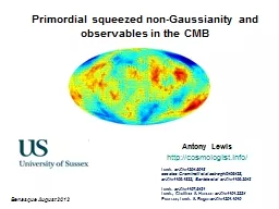
PPT-Primordial squeezed non-Gaussianity and observables in the PowerPoint Presentation

Antony Lewis httpcosmologistinfo Lewis arXiv12045018 see also Creminelli et al astroph 0405428 arXiv11091822 Bartolo et al arXiv11092043 Lewis arXiv11075431

Upload by sherrill-nordquist
Published on 2016-07-18

Presentation Embed Code

<iframe width="560" height="315" src="https://www.docslides.com/embed/410223" frameborder="0" allowfullscreen></iframe>

Download Presentation

Download Presentation The PPT/PDF document "Primordial squeezed non-Gaussianity and ..." is the property of its rightful owner. Permission is granted to download and print the materials on this web site for personal, non-commercial use only, and to display it on your personal computer provided you do not modify the materials and that you retain all copyright notices contained in the materials. By downloading content from our website, you accept the terms of this agreement.