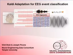
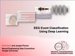
Neural Engineering Data Consortium Temple University EEG Event Classification Using Deep Learning What is an EEG Electroencephalography EEG is a popular tool used to diagnose brain related illnesses ID: 774759
Download Presentation The PPT/PDF document " Vinit Shah and Joseph Picone" is the property of its rightful owner. Permission is granted to download and print the materials on this web site for personal, non-commercial use only, and to display it on your personal computer provided you do not modify the materials and that you retain all copyright notices contained in the materials. By downloading content from our website, you accept the terms of this agreement.
Slide1
Vinit Shah and Joseph PiconeNeural Engineering Data ConsortiumTemple University
EEG Event Classification
Using Deep Learning
Slide2What is an EEG ?
Electroencephalography (EEG) is a popular tool used to diagnose brain related illnesses.
Scalp Electroencephalogram (EEG) monitoring is a non-invasive and convenient method to assess electrical activity from brain.
Interpretation of EEGs is challenging, and its accurate annotation requires extensive training.
Diagnosis is performed considering the factors such as patient’s record video, history, age, environmental & physiological changes, etc.
Slide3Seizure Morphologies
Electrographic seizures can be detected either by observing epileptiform activities or by observing artifacts related to specific types of seizures.
There are multiple types of seizures (i.e. Tonic-
Clonic
/Grand mal, Absence/Petit mal, complex-partial)
Interpretation of focal seizures require temporal as well as sufficient level of spatial information.
Typically interpreters look for epileptiform activity such as spike and wave discharges and its evolution over time.
Easy seizures show clear evolution in signal’s frequency and amplitude.
Slide4Inconclusive Segments
Some EEG records are very challenging and show wide spread epileptiform features along with artifacts (i.e. Shivers). Obscured patterns as such could also make interpretation inconclusive in some cases.
Accurate onset and offset detection of an ictal is in many cases subjective which encourages us to use Any-Overlap method for scoring.
Shivers
Epileptiform
Activity
Slide5Spectral Properties of an Ictal Seizure
Seizures usually occur within the range of 2.5 to 25 Hz.
Seizure duration can rand from 3 seconds to days.
Generalized seizures are easy to spot dueto their high energyin specificfrequency bands.Waxing-waning patterns (e.g., bursts) can be mistakenly identified as ictal.
Slide6Artifacts and Medications Pose Challenges
Artifacts such as chewing resemble features of tonic-clonic and complex-partial seizures.
This is usually disambiguated from the context/history of the record.
Medication makes it more difficult.Subtle seizures such as extremely focal, low energy seizures are widespread in ICU patients due to medication.
Slide7Feature Extraction
Version 1.2.1Training setEvaluation setw/seizTotalw/seizTotalPatients1192653850Sessions18258398239Epochs(sec.)76,517(6.4%)1,196,381(100.0%)55,765(9.0%)618,096(100.0%)
TUH EEG Seizure Corpus (v1.2.1) was used:The database consists of clinical data with many types of seizures and lots of artifacts.World’s largest open source repository of EEG data.
Standard frequency domain features are used:
10 frames per second
0.2 second analysis window
9 base features including energy, differential energy, and 7 cepstral coefficients.
1st and 2nd derivatives are used for most features.
Total dimension: 26.
Slide8Baseline System: CNN-LSTM
Three baseline systems:CNN-LSTM systemChannel based LSTM networksA Kaldi multipass system with P-norm and MLP networks.
CNN-LSTM Model
CNN-LSTM Architecture:
Each sample is a 21 sec. long window for all 22 channels.
Trained with constant learning rate with a kernel size of (3, 3).
Heuristic postprocessing approaches are applied which include a threshold for output probabilities and seizure events of a certain duration.
An Adam optimizer is used.
Slide9LSTM Model
Baseline System: LSTM
Channel based LSTM Architecture:
Each sample is a 7 sec. long
window with right/left context
(splice width) of 11 frames
(1.1 sec.).
Each channel is processed
individually so that the model
only learns spike/sharp and wave
discharges.
Trained with annealing learning
rate after CV loss is stagnated
for 3 consecutive epochs.
SGD optimizer with
nestrov
momentum is used.
A small CNN-LSTM-MLP model is used for postprocessing followed by heuristic postprocessing.
Slide10Baseline System: Kaldi
Kaldi baseline systems:Kaldi multipass systems with P-norm (Dan’s DNN (nnet2) implementation)Kaldi multipass systems with MLP networks (TF implementation).
Kaldi P-norm fast:
Fixed Affined Component / LDA is applied to decorrelate splice window of 11 (Left/Right context of 5).Training is performed for 20 epochs with annealing learning rate with last 5 epochs with constant minimum lr.P-norm Input dim = 2000 & Output dim = 400.Preconditioned SGD is used which is a matrix valued learning rate.
Kaldi DNN (TF):
Tensorflow’s
MLP network with 3 hidden layers
is implemented.
Priors, decision tree and alignments from Kaldi’s LDA-MLLT systems are used for acoustic modeling.
Slide11Evaluation Metrics
Any Overlap method (OVLP):
Any overlap method is a permissive method which looks for the detection of an event within a proximity of the reference.This metric tend to produce higher sensitivitiessince only isolated events are considered as false alarms.Multiple overlapping events detected in bursts are also counts towards detection.
Performance measures are calculated in terms of Sensitivity and Specificity (or false alarms per 24 hours):
Sensitivity = ( True Positives / (True Positives + False Negatives) )
Specificity = (True Negatives / (True Negatives + False Positives)
)
False Alarm rate = Rate of ( ( # Target False Positives / Total duration ) × (60 × 60 × 24) )
Slide12Performance
DNN ModelSensitivity (%)FA/24 HoursCNN-LSTM30.8%6.7%LSTM 40.3% 5.8%Kaldi P-Norm 60.1% 25.7%Kaldi MLP 49.8% 2.6%
Kaldi models use word boundary information during event classification.Kaldi’s best performance is only ~50% sensitivity @ 2.58 FAs/24 hours (with word boundaries).Channel-based LSTM network outperforms other models with no word boundary information.
ROC curve for the target/seizure class.
The region of interest is when the FA is low (< 10 FAs/24 hours).
Slide13Decoding and Error Analysis
Kaldi lattices were used during decoding.Lattice-1best, lattice-push and lattice-to-post were used to obtain decoding results. Each of which uses word boundaries.Kaldi has a crude energy based automatic segmentation approach which is not adequate for segmentation of EEGs.
Reference Transcriptions
Hypothesis Transcriptions
Slide14P-Norm DNN (Kaldi)
Posterior Distribution
LSTM network (
AutoEEG
)
Decoding and Error Analysis
Performance of the DNN-HMM models on seizures with different durations is quite similar. Decoded transcription probabilities are very high compared to any non-Kaldi models we have developed.Due to the binary classification problem, LM seems to flip the correctly detect classes at the beginning and end of the record.