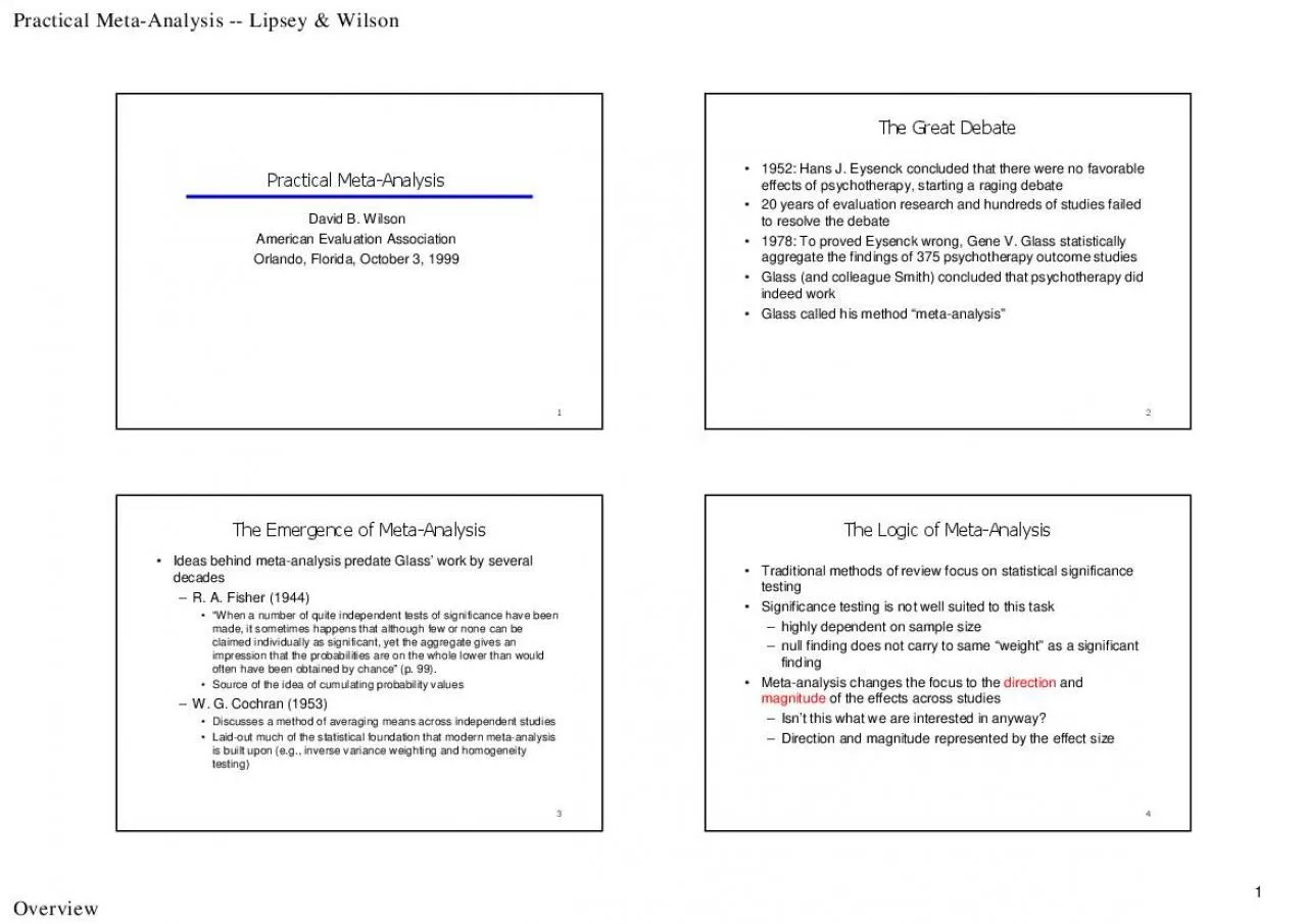
Practical MetaAnalysis Lipsey WilsonOverview - PDF document

1 Practical Meta-Analysis --Lipsey & Wilso
Practical Meta-Analysis --Lipsey & WilsonOverview Practical Meta-AnalysisDavid B. WilsonAmerican Evaluation AssociationOrlando, Florida, October 3, 1999 The Great Debate1952: Hans J. Eysenck concluded that there were no favorableeffects of psychotherapy, starting a raging debate20 years of evaluation research and hundreds of studies failedto resolve the debate1978: To proved Eysenck wrong, Gene V. Glass statisticallyaggregate the findings of 375 psychotherapy outcome studiesGlass (and colleague Smith) concluded that psychotherapy didindeed workGlass called his method “meta-analysis” The Emergence of Meta-AnalysisIdeas behind meta-analysis predate Glass’work by severaldecades–R. A. Fisher (1944)“When a number of quite independent tests of significance have beenmade, it sometimes happens that although few or none can beclaimed individually as significant, yet the aggregate gives animpression that the probabilities are on the whole lower than wouldoften have been obtained by chance”(p. 99).Source of the idea of cumulating probability values–W. G. Cochran (1953)Discusses a method of averaging means across independent studiesLaid-out much of the statistical foundation that modern meta-analysisis built upon (e.g., inverse variance weighting and homogeneitytesting) The Logic of Meta-Analysi

2 sTraditional methods of review focus on
sTraditional methods of review focus on statistical significancetestingSignificance testing is not well suited to this task–highly dependent on sample size–null finding does not carry to same “weight”as a significantfindingMeta-analysis changes the focus to thedirectionandmagnitudeof the effects across studies–Isn’t this what we are interested in anyway?–Direction and magnitude represented by the effect size Practical Meta-Analysis --Lipsey & WilsonOverview When Can You Do Meta-Analysis?Meta-analysis is applicable to collections of research that–are empirical, rather than theoretical–produce quantitative results, rather than qualitative findings–examine the same constructs and relationships–have findings that can be configured in a comparablestatistical form (e.g., as effect sizes, correlation coefficients,odds-ratios, etc.)–are “comparable”given the question at hand Forms of Research Findings Suitable to Meta-AnalysisCentral Tendency Research–prevalence ratesPre-Post Contrasts–growth ratesGroup Contrasts–experimentally created groupscomparison of outcomes between treatment and comparison groups–naturally occurring groupscomparison of spatial abilities between boys and girlsAssociation Between Variables–measurement researchvalidity generalization–individual differences researchcorr

3 elation between personality constructs E
elation between personality constructs Effect Size: The Key to Meta-AnalysisThe effect size makes meta-analysis possible–it is the “dependent variable”–it standardizes findings across studies such that they can bedirectly comparedAny standardized index can be an “effect size”(e.g.,standardized mean difference, correlation coefficient, odds-ratio) as long as it meets the following–is comparable across studies (generally requiresstandardization)–represents the magnitude and direction of the relationship ofinterest–is independent of sample sizeDifferent meta-analyses may use different effect size indices The Replication Continuum PureReplicationsConceptualReplicationsYou must be able to argue that the collection of studies you aremeta-analyzing examine the same relationship. This may be at a broadlevel of abstraction, such as the relationship between criminal justiceinterventions and recidivism or between school-based preventionprograms and problem behavior. Alternatively it may be at a narrowlevel of abstraction and represent pure replications.The closer to pure replications your collection of studies, the easier itis to argue comparability. Practical Meta-Analysis --Lipsey & WilsonOverview Which Studies to Include?It is critical to have an explicit inclusion and exclusion criteria(see han

4 dout)–the broader the research domain, t
dout)–the broader the research domain, the more detailed theytend to become–developed iteratively as you interact with the literatureTo include or exclude low quality studies–the findings of all studies are potentially in error(methodological quality is a continuum, not a dichotomy)–being too restrictive may restrict ability to generalize–being too inclusive may weaken the confidence that can beplaced in the findings–must strike a balance that is appropriate to your researchquestion Searching Far and WideThe “we only included published studies because they havebeen peer-reviewed”argumentSignificant findings are more likely to be published thannonsignificant findingsCritical to try to identify and retrieve all studies that meet youreligibility criteriaPotential sources for identification of documents–computerized bibliographic databases–authors working in the research domain–conference programs–dissertations–review articles–hand searching relevant journal–government reports, bibliographies, clearinghouses Strengths of Meta-AnalysisImposes a discipline on the process of summing up researchfindingsRepresents findings in a more differentiated and sophisticatedmanner than conventional reviewsCapable of finding relationships across studies that areobscured in other approachesProtects again

5 st over-interpreting differences across
st over-interpreting differences across studiesCan handle a large numbers of studies (this would overwhelmtraditional approaches to review) Weaknesses of Meta-AnalysisRequires a good deal of effortMechanical aspects don’t lend themselves to capturing morequalitative distinctions between studies“Apples and oranges”; comparability of studies is often in the“eye of the beholder”Most meta-analyses include “blemished”studiesSelection bias posses continual threat–negative and null finding studies that you were unable tofind–outcomes for which there were negative or null findings thatwere not reportedAnalysis of between study differences is fundamentallycorrelational Practical Meta-Analysis --Lipsey & WilsonEffect Size Overheads The Effect SizeThe effect size (ES) makes meta-analysis possible.The ES encodes the selected research findings on anumeric scale.There are many different types of ES measures, eachsuited to different research situations.Each ES type may also have multiple methods ofcomputation. Examples of Different Types of Effect Sizes:The Major LeaguesStandardized Mean Difference–group contrast researchtreatment groupsnaturally occurring groups–inherently continuous constructOdds-Ratio–group contrast researchtreatment groupsnaturally occurring groups–inherently dichotomous

6 constructCorrelation Coefficient–assoc
constructCorrelation Coefficient–association between variables research Examples of Different Types of Effect Sizes:Two from the Minor LeaguesProportion–central tendency researchHIV/AIDS prevalence ratesProportion of homeless persons found to be alcohol abusersStandardized Gain Score–gain or change between two measurement points on the samevariablereading speed before and after a reading improvement class What Makes Something an Effect Sizefor Meta-Analytic PurposesThe type of ES must be comparable across the collectionof studies of interest.This is generally accomplished through standardization.Must be able to calculate a standard error for that type of–the standard error is needed to calculate the ES weights, calledinverse variance weights (more on this latter)–all meta-analytic analyses are weighted Practical Meta-Analysis --Lipsey & WilsonEffect Size Overheads The Standardized Mean DifferenceRepresents a standardized group contrast on aninherently continuousmeasure.Uses the pooled standard deviation (some situations usecontrol group standard deviation).Commonly called “d”or occasionally “g”. pooled pooled The Correlation CoefficientRepresents the strength of association between twoinherently continuousmeasures.Generally reported directly as “r”(the Pearson productmoment coef

7 ficient). rES The Odds-RatioThe Odds-Ra
ficient). rES The Odds-RatioThe Odds-Ratio is based on a 2 by 2 contingency table,such as the one below.Frequencies Success FailureTreatment GroupControl Group bc The Odds-Ratio is the odds of success in the treatmentgroup relative to the odds of success in the control group. Methods of Calculating theStandardized Mean DifferenceThe standardized mean difference probably has moremethods of calculation than any other effect size type. Practical Meta-Analysis --Lipsey & WilsonEffect Size Overheads The different formulas represent degrees of approximation tothe ES value that would be obtained based on the means andstandard deviations–direct calculation based on means and standard deviations–algebraically equivalent formulas (t-test)–exact probability value for a t-test–approximations based on continuous data (correlation coefficient)–estimates of the mean difference (adjusted means, regression Bweight, gain score means)–estimates of the pooled standard deviation (gain score standarddeviation, one-way ANOVA with 3 or more groups, ANCOVA)–approximations based on dichotomous dataGreatPoor Methods of Calculating theStandardized Mean Difference pooledDirection Calculation Method Methods of Calculating theStandardized Mean Difference Algebraically Equivalent Formulas: independent t-testtwo-group one-

8 way ANOVAexactp-values-test or-ratio can
way ANOVAexactp-values-test or-ratio can be convertedinto-value and the above formula applied Methods of Calculating theStandardized Mean DifferenceA study may report a grouped frequency distributionfrom which you can calculate means and standarddeviations and apply to direct calculation method. Practical Meta-Analysis --Lipsey & WilsonEffect Size Overheads Methods of Calculating theStandardized Mean Difference Close Approximation Based on Continuous Data --Point-Biserial Correlation. For example, the correlationbetween treatment/no treatment and outcome measuredon a continuous scale. Methods of Calculating theStandardized Mean DifferenceEstimates of the Numerator of ES --The Mean Difference--difference between gain scores--difference between covariance adjusted means--unstandardized regression coefficient for group membership Methods of Calculating theStandardized Mean DifferenceEstimates of the Denominator of ES --Pooled Standard Deviation pooledstandard error of the mean Methods of Calculating theStandardized Mean DifferenceEstimates of the Denominator of ES --Pooled Standard Deviation betweenpooled 1 )(22 k betweenone-way AN�OVA 2 groups Practical Meta-Analysis --Lipsey & WilsonEffect Size Overheads Methods of Calculating theStandardized Mean DifferenceEstimates of the Denominator

9 of ES --Pooled Standard Deviation gainpo
of ES --Pooled Standard Deviation gainpooledstandard deviation of gainscores, whereis the correlationbetween pretest and posttestscores Methods of Calculating theStandardized Mean DifferenceEstimates of the Denominator of ES --Pooled Standard Deviation pooledANCOVA, whereis thecorrelation between thecovariate and the DV Methods of Calculating theStandardized Mean DifferenceEstimates of the Denominator of ES --Pooled Standard Deviation pooledA two-way factorial ANOVAwhere B is the irrelevant factorand AB is the interactionbetween the irrelevant factorand group membership (factor Methods of Calculating theStandardized Mean DifferenceApproximations Based on Dichotomous Datagroupgroupthe difference between the probits transformationof the proportion successful in each groupconverts proportion into a-value Practical Meta-Analysis --Lipsey & WilsonEffect Size Overheads Methods of Calculating theStandardized Mean DifferenceApproximations Based on Dichotomous Data chi-square must be based ona 2 by 2 contingency table(i.e., have only 1 df) phi coefficient 22 23 Formulas for the Correlation CoefficientResults typically reported directly as a correlation.Any data for which you can calculate a standardized meandifference effect size, you can also calculate a correlationtype effect size.See Appendix B f

10 or formulas. Practical Meta-Analysis --L
or formulas. Practical Meta-Analysis --Lipsey & WilsonEffect Size Overheads Formulas for the Odds RatioResults typically reported in one of three forms:–frequency of successes in each group–proportion of successes in each group–2 by 2 contingency tableAppendix B provides formulas for each situation. Data to Code Along with the ESThe Effect Size–may want to code the data from which the ES is calculated–confidence in ES calculation–method of calculation–any additional data needed for calculation of the inverse varianceweightSample SizeES specific attritionConstruct measuredPoint in time when variable measuredReliability of measureType of statistical test used Practical Meta-Analysis --Lipsey & WilsonAnalysis Overheads Overview of Meta-Analytic Data AnalysisTransformations, Adjustments and OutliersThe Inverse Variance WeightThe Mean Effect Size and Associated StatisticsHomogeneity AnalysisFixed Effects Analysis of Heterogeneous Distributions–Fixed Effects Analog to the one-way ANOVA–Fixed Effects Regression AnalysisRandom Effects Analysis of Heterogeneous Distributions–Mean Random Effects ES and Associated Statistics–Random Effects Analog to the one-way ANOVA–Random Effects Regression Analysis TransformationsSome effect size types are not analyzed in their “raw”form.Standardized

11 Mean Difference Effect Size–Upward bias
Mean Difference Effect Size–Upward bias when sample sizes are small–Removed with the small sample size bias correction 9431'NESESsmsm Transformations (continued)Correlation has a problematic standard error formula.Recall that the standard error is needed for the inversevariance weight.Solution: Fisher’s Zr transformation.Finally results can be converted back into “r”with theinverse Zr transformation (see Chapter 3). Transformations (continued)Analyses performed on the Fisher’s Zr transformedcorrelations.Finally results can be converted back into “r”with theinverse Zr transformation. rrESZr11ln5. 1 122ZrZrESES e er Practical Meta-Analysis --Lipsey & WilsonAnalysis Overheads Transformations (continued)Odds-Ratio is asymmetric and has a complex standarderror formula.–Negative relationships indicated by values between 0 and 1.–Positive relationships indicated by values between 1 and infinity.Solution: Natural log of the Odds-Ratio.–Negative relationship 0.–No relationship = 0.–Positive relationsh&#x -40;ip 0.Finally results can be converted back into Odds-Ratios bythe inverse natural log function. Transformations (continued)Analyses performed on the natural log of the Odds-Ratio:Finally results converted back via inverse natural logfunction: LOR AdjustmentsHunter and Schmidt Artifact

12 Adjustments–measurement unreliability (n
Adjustments–measurement unreliability (need reliability coefficient)–range restriction (need unrestricted standard deviation)–artificial dichotomization (correlation effect sizes only)assumes a normal underlying distributionOutliers–extreme effect sizes may have disproportionate influence onanalysis–either remove them from the analysis or adjust them to a lessextreme value–indicate what you have done in any written report Overview of Transformations, Adjustments,and OutliersStandard transformations–sample sample size bias correction for the standardized meandifference effect size–Fisher’s Z to r transformation for correlation coefficients–Natural log transformation for odds-ratiosHunter and Schmidt Adjustments–perform if interested in what would have occurred under “ideal”research conditionsOutliers–any extreme effect sizes have been appropriately handled Practical Meta-Analysis --Lipsey & WilsonAnalysis Overheads Independent Set of Effect SizesMust be dealing with an independent set of effect sizesbefore proceeding with the analysis.–One ES per study OR–One ES per subsample within a study The Inverse Variance WeightStudies generally vary in size.An ES based on 100 subjects is assumed to be a more“precise”estimate of the population ES than is an ESbased on 10 subjects.Therefore, large

13 r studies should carry more “weight”in o
r studies should carry more “weight”in ouranalyses than smaller studies.Simple approach: weight each ES by its sample size.Better approach: weight by the inverse variance. What is the Inverse Variance Weight?The standard error (SE) is a direct index of ES precision.SE is used to create confidence intervals.The smaller the SE, the more precise the ES.Hedges’showed that the optimal weights for meta-analysis are: 21 SE w Inverse Variance Weight for theThree Major League Effect SizesStandardized Mean Difference: 21 se w Zr transformed Correlation Coefficient: nw 31nse Practical Meta-Analysis --Lipsey & WilsonAnalysis Overheads Inverse Variance Weight for theThree Major League Effect SizesLogged Odds-Ratio: 21 se w Where a, b, c, and d are the cell frequencies of a 2 by 2contingency table. Ready to AnalyzeWe have an independent set of effect sizes (ES) that havebeen transformed and/or adjusted, if needed.For each effect size we have an inverse variance weight The Weighted Mean Effect SizeStart with the effect size(ES) and inverse varianceweight (w) for 10 studies. Study-0.3311.910.3228.570.3958.820.3129.410.1713.890.648.55-0.339.800.1510.75-0.0283.330.0014.93 wESwES)( The Weighted Mean Effect SizeStart with the effect size(ES) and inverse varianceweight (w) for 10 studies.Next, mult

14 iply w by ES. Studyw*ES-0.3311.91-3.930.
iply w by ES. Studyw*ES-0.3311.91-3.930.3228.570.3958.820.3129.410.1713.890.648.55-0.339.800.1510.75-0.0283.330.0014.93 Practical Meta-Analysis --Lipsey & WilsonAnalysis Overheads The Weighted Mean Effect SizeStart with the effect size(ES) and inverse varianceweight (w) for 10 studies.Next, multiply w by ES.Repeat for all effect sizes. Studyw*ES-0.3311.91-3.930.3228.579.140.3958.8222.940.3129.419.120.1713.892.360.648.555.47-0.339.80-3.240.1510.751.61-0.0283.33-1.670.0014.930.00 The Weighted Mean Effect SizeStart with the effect size (ES)and inverse variance weight(w) for 10 studies.Next, multiply w by ES.Repeat for all effect sizes.Sum the columns, w and ES.Divide the sum of (w*ES) bythe sum of (w). Studyw*ES-0.3311.91-3.930.3228.579.140.3958.8222.940.3129.419.120.1713.892.360.648.555.47-0.339.80-3.240.1510.751.61-0.0283.33-1.670.0014.930.00269.9641.82 15.096.26982.41)( wESwES The Standard Error of the Mean ESThe standard error of themean is the square root of1 divided by the sum ofthe weights. Studyw*ES-0.3311.91-3.930.3228.579.140.3958.8222.940.3129.419.120.1713.892.360.648.555.47-0.339.80-3.240.1510.751.61-0.0283.33-1.670.0014.930.00269.9641.82 061.096.26911wseES Mean, Standard Error,Z-test and Confidence Intervals 15.096.26982.41)( wESwES 061.096.26911wseES 46.2061.015.0ESseESZ 27

15 .0)061(.96.115.0)(96.1ESseESUpper LowerM
.0)061(.96.115.0)(96.1ESseESUpper LowerMean ESSE of the Mean ESZ-test for the Mean ES95% Confidence Interval Practical Meta-Analysis --Lipsey & WilsonAnalysis Overheads Homogeneity AnalysisHomogeneity analysis tests whether the assumption thatall of the effect sizes are estimating the same populationmean is a reasonable assumption.If homogeneity is rejected, the distribution of effect sizes isassumed to be heterogeneous.–Single mean ES not a good descriptor of the distribution–There are real between study differences, that is, studies estimatedifferent population mean effect sizes.–Two options:model between study differencesfit a random effects model Q -The Homogeneity StatisticCalculate a new variablethat is the ES squaredmultiplied by the weight.Sum new variable. Studyw*ESw*ES^2-0.3311.91-3.931.300.3228.579.142.930.3958.8222.948.950.3129.419.122.830.1713.892.360.400.648.555.473.50-0.339.80-3.241.070.1510.751.610.24-0.0283.33-1.670.030.0014.930.000.00269.9641.8221.24 Calculating QWe now have 3 sums: 76.1448.624.2196.26982.4124.21)(222 wESwESwQ24.21)(82.41)(96.2692 Q is can be calculated using these 3 sums: Interpreting QQ is distributed as a Chi-Squaredf = number of ESs -1Running example has 10 ESs, therefore, df = 9Critical Value for a Chi-Square with df = 9 and p = .05 is:Since o

16 ur Calculated Q (14.76) is less than 16.
ur Calculated Q (14.76) is less than 16.92, wefail to reject the null hypothesis of homogeneity.Thus, the variability across effect sizes does not exceedwhat would be expected based on sampling error.16.92 Practical Meta-Analysis --Lipsey & WilsonAnalysis Overheads Heterogeneous Distributions: What Now?Analyze excess between study (ES) variability–categorical variables with the analog to the one-way ANOVA–continuous variables and/or multiple variables with weightedmultiple regressionAssume variability is random and fit a random effectsmodel. Analyzing Heterogeneous Distributions:The Analog to the ANOVACalculate the 3 sumsfor each subgroup ofeffect sizes. StudyGrpw*ESw*ES^2-0.3311.91-3.931.300.3228.579.142.930.3958.8222.948.950.3129.419.122.830.1713.892.360.400.648.555.473.50151.1545.1019.90-0.339.80-3.241.070.1510.751.610.24-0.0283.33-1.670.030.0014.930.000.00118.82-3.291.34 A grouping variable (e.g., random vs. nonrandom) Analyzing Heterogeneous Distributions:The Analog to the ANOVACalculate a separate Q for each group: 44.615.15110.4590.1921_GROUPQ 25.182.11829.334.122_GROUPQ Analyzing Heterogeneous Distributions:The Analog to the ANOVAThe sum of the individual group Qs = Q within:The difference between the Q total and the Q withinis the Q between: Where k is the number of effect sizesan

17 d j is the number of groups. Where j is
d j is the number of groups. Where j is the number of groups. Practical Meta-Analysis --Lipsey & WilsonAnalysis Overheads Analyzing Heterogeneous Distributions:The Analog to the ANOVAAll we did was partition the overall Q into two pieces, awithin groups Q and a between groups Q. The grouping variable accounts for significant variabilityin effect sizes. Mean ES for each GroupThe mean ES, standard error and confidence intervalscan be calculated for each group: 30.015.15110.45)(1_ wESwESGROUP 03.082.11829.3)(2_ wESwESGROUP Analyzing Heterogeneous Distributions:Multiple Regression AnalysisAnalog to the ANOVA is restricted to a single categoricalbetween studies variable.What if you are interested in a continuous variable ormultiple between study variables?Weighted Multiple Regression Analysis–as always, it is weighted analysis–can use “canned”programs (e.g., SPSS, SAS)parameter estimates are correct (R-squared, B weights, etc.)F-tests, t-tests, and associated probabilities areincorrect –can use Wilson/Lipsey SPSS macros which give correctparameters and probability values Meta-Analytic Multiple Regression ResultsFrom the Wilson/Lipsey SPSS Macro(data set with 39 ESs)***** Meta-Analytic Generalized OLS Regression *****-------Homogeneity Analysis -------Q df pModel 1

18 04.9704 3.0000 .0000Residua
04.9704 3.0000 .0000Residual 424.6276 34.0000 .0000-------Regression Coefficients -------B SE -95% CI +95% CI Z P BetaConstant -.7782 .0925 -.9595 -.5970 -8.4170 .0000 .0000RANDOM .0786 .0215 .0364 .1207 3.6548 .0003 .1696TXVAR1 .5065 .0753 .3590 .6541 6.7285 .0000 .2933TXVAR2 .1641 .0231 .1188 .2094 7.1036 .0000 .3298Partition of total Q into varianceexplained by the regression“model”and the variance left over(“residual”). Interpretation is the same as will ordinal multiple regression analysis. If residual Q is significant, fit a mixed effects model. Practical Meta-Analysis --Lipsey & WilsonAnalysis Overheads Review of WeightedMultiple Regression AnalysisAnalysis is weighted.Q for the model indicates if the regression model explainsa significant portion of the variability across effect sizes.Q for the residual indicates if the remaining variabilityacross effect sizes is homogeneous.If using a “canned”regression program, must correct theprobability values (see manuscript for details). Random Effects ModelsDon’t panic!It sounds far worse than it is.Three reasons to use a random effects model–Total Q is significant and you assume that the excess variabilityacr

19 oss effect sizes derives from random dif
oss effect sizes derives from random differences across studies(sources you cannot identify or measure).–The Q within from an Analog to the ANOVA is significant.–The Q residual from a Weighted Multiple Regression analysis issignificant. The Logic of aRandom Effects ModelFixed effects model assumes that all of the variabilitybetween effect sizes is due to sampling error.Random effects model assumes that the variabilitybetween effect sizes is due to sampling errorplusvariability in the population of effects (unique differencesin the set of true population effect sizes). The Basic Procedure of aRandom Effects ModelFixed effects model weights each study by the inverse ofthe sampling variance.Random effects model weights each study by the inverseof the sampling varianceplusa constant that representsthe variability across the population effects. 21iisew vsewiiˆ12 This is the random effects variancecomponent. Practical Meta-Analysis --Lipsey & WilsonAnalysis Overheads How To Estimate the RandomEffects Variance ComponentThe random effects variance component is based on Q.The formula is: wwwkQvT2)1(ˆ Calculation of the RandomEffects Variance ComponentCalculate a newvariable that is thew squared.Sum new variable. Studyw*ESw*ES^2w^2-0.3311.91-3.931.30141.730.3228.579.142.93816.300.3958.8222.948.9

20 53460.260.3129.419.122.83865.070.1713.89
53460.260.3129.419.122.83865.070.1713.892.360.40192.900.648.555.473.5073.05-0.339.80-3.241.0796.120.1510.751.610.24115.63-0.0283.33-1.670.036944.390.0014.930.000.00222.76269.9641.8221.2412928.21 Calculation of the RandomEffects Variance ComponentThe total Q for this data was 14.76k is the number of effect sizes (10)The sum of w = 269.96The sum of w= 12,928.21 026.089.4796.26976.596.26921.928,1296.269)110(76.14)1(ˆ2 wwwkQvT Rerun Analysis with NewInverse Variance WeightAdd the random effects variance component to thevariance associated with each ES.Calculate a new weight.Rerun analysis.Congratulations! You have just performed a very complexstatistical analysis. vsewiiˆ12 Practical Meta-Analysis --Lipsey & WilsonAnalysis Overheads Random Effects Variance Componentfor the Analog to the ANOVA andRegression AnalysisThe Q between or Q residual replaces the Q total in theformula.Denominator gets a little more complex and relies onmatrix algebra. However, the logic is the same.SPSS macros perform the calculation for you. SPSS Macro Output with Random EffectsVariance Component-------Homogeneity Analysis -------Q df pModel 104.9704 3.0000 .0000Residual 424.6276 34.0000 .0000-------Regression Coefficients -------B SE -95% CI +9

21 5% CI Z P BetaConstant
5% CI Z P BetaConstant -.7782 .0925 -.9595 -.5970 -8.4170 .0000 .0000RANDOM .0786 .0215 .0364 .1207 3.6548 .0003 .1696TXVAR1 .5065 .0753 .3590 .6541 6.7285 .0000 .2933TXVAR2 .1641 .0231 .1188 .2094 7.1036 .0000 .3298-------Estimated Random Effects Variance Component -------Not included in above model which is a fixed effects model Random effects variance component based on the residual Q. Add thisvalue to each ES variance (SE squared) and recalculate w. Rerunanalysiswith the new w. Comparison of Random Effect withFixed Effect ResultsThe biggest difference you will notice is in the significancelevels and confidence intervals.–Confidence intervals will get bigger.–Effects that were significant under a fixed effect model may nolonger be significant.Random effects models are therefore more conservative. Review of Meta-Analytic Data AnalysisTransformations, Adjustments and OutliersThe Inverse Variance WeightThe Mean Effect Size and Associated StatisticsHomogeneity AnalysisFixed Effects Analysis of Heterogeneous Distributions–Fixed Effects Analog to the one-way ANOVA–Fixed Effects Regression AnalysisRandom Effects Analysis of Heterogeneous Distributions–Mean Random Effects ES and Associated Statis

22 tics–Random Effects Analog to the one-wa
tics–Random Effects Analog to the one-way ANOVA–Random Effects Regression Analysis Practical Meta-Analysis --Lipsey & WilsonInterpretation Overheads Interpreting Effect Size ResultsCohen’s “Rules-of-Thumb”–standardized mean difference effect sizesmall = 0.20medium = 0.50large = 0.80–correlation coefficientsmall = 0.10medium = 0.25large = 0.40–odds-ratiosmall = 1.50medium = 2.50large = 4.30These do not take into account the context of the interventionThey do correspond to the distribution of effects across meta-analyses found by Lipsey and Wilson (1993) Interpreting Effect Size ResultsRules-of-Thumb do not take into account the context of theintervention–a “small”effect may be highly meaningful for an interventionthat requires few resources and imposes little on theparticipants–small effects may be more meaningful for serious and fairlyintractable problemsCohen’s Rules-of-Thumb do, however, correspond to thedistribution of effects across meta-analyses found by Lipseyand Wilson (1993) Translation of Effect SizesOriginal metricSuccess Rates (Rosenthal and Rubin’s BESD)–Proportion of “successes”in the treatment and comparisongroups assuming an overall success rate of 50%–Can be adapted to alternative overall success ratesExample using the sex offender data–Assuming a comparison gr

23 oup recidivism rate of 15%, theeffect si
oup recidivism rate of 15%, theeffect size of 0.45 for the cognitive-behavioral treatmentstranslates into a recidivism rate for the treatment group of Methodological Adequacy of Research BaseFindings must be interpreted within the bounds of themethodological quality of the research base synthesized.Studies often cannot simply be grouped into “good”and “bad”studies.Some methodological weaknesses may bias the overallfindings, others may merely add “noise”to the distribution. Practical Meta-Analysis --Lipsey & WilsonInterpretation Overheads Confounding of Study FeaturesRelative comparisons of effect sizes across studies areinherently correlational!Important study features are often confounding, obscuring theinterpretive meaning of observed differencesIf the confounding is not severe and you have a sufficientnumber of studies, you can model “out”the influence of methodfeatures to clarify substantive differences Concluding CommentsMeta-analysis is a replicable and defensible method ofsynthesizing findings across studiesMeta-analysis often points out gaps in the research literature,providing a solid foundation for the next generation of researchon that topicMeta-analysis illustrates the importance of replicationMeta-analysis facilitates generalization of the knowledge gainthrough individua