/
Sensitivity of Squall-Line Rear Inflow to Ice Microphysics Sensitivity of Squall-Line Rear Inflow to Ice Microphysics

Sensitivity of Squall-Line Rear Inflow to Ice Microphysics - PowerPoint Presentation

stefany-barnette
stefany-barnette . @stefany-barnette
Follow
434 views
Uploaded On 2017-01-11

Sensitivity of Squall-Line Rear Inflow to Ice Microphysics - PPT Presentation

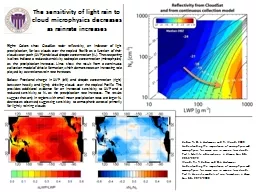
Yang MJ and RA Houze Jr RTF Hydrometeor types Icephase microphysics Environmental humidity No 1 microphysics processes CNTL Full model physics for 15 h Turn off the hail generation processes after 6 h ID: 508447

storm rtf region line rtf storm line region cloud hail flow microphysics cntl weaker cooling tilt ice precipitation upshear

Share:

Link:

Embed:

Download Presentation from below link

Download Presentation The PPT/PDF document "Sensitivity of Squall-Line Rear Inflow t..." is the property of its rightful owner. Permission is granted to download and print the materials on this web site for personal, non-commercial use only, and to display it on your personal computer provided you do not modify the materials and that you retain all copyright notices contained in the materials. By downloading content from our website, you accept the terms of this agreement.


Presentation Transcript

Slide1

Sensitivity of Squall-Line Rear Inflow to Ice Microphysics and Environmental Humidity

Yang, M.-J., and R.A.

Houze

,

JrSlide2

RTF

Hydrometeor types

Ice-phase microphysics

Environmental humidity

No. 1 microphysics processesSlide3

CNTL

Full model physics for 15 h.

Turn off the hail generation processes after 6 h (Fovell and Ogura, 1988), because there were very few hailstones in the mature or decaying stage of the 10-11 June squall line.Slide4

CNTL – Overview

Hail offSlide5

initial

mature

decayingSlide6

initial

mature

decaying

Shaded:

Cloud region

(

no

rain, mixing ratial > 0.1 g/kg)Highlighted:

Storm Precipitation boundary (radar reflectivity of 15 dBZ)

Line:

storm-relative horizontal wind field

(dash line: FTR; solid line: RTF)

Kinematic

Structure

FTR

RTFSlide7

Shaded:

Cloud region

(

no

rain, mixing ratial > 0.1 g/kg)Highlighted: Storm Precipitation boundary

(radar reflectivity of 15 dBZ)Line: Vertical velocity

(dash line: ↓; solid line: ↑)Slide8

Shaded:

Cloud region

(

no

rain, mixing ratial > 0.1 g/kg)Highlighted: Storm Precipitation boundary

(radar reflectivity of 15 dBZ)Line: Potential temperature perturbation(dash line: - ; solid line: +)

Thermal and Pressure

Structure

warm

coolSlide9

Shaded:

Cloud region

(

no

rain, mixing ratial > 0.1 g/kg)Highlighted: Storm Precipitation boundary

(radar reflectivity of 15 dBZ)Line: Pressure perturbation field(dash line: - ; solid line: +)Slide10

Heating:

Condensation of cloud water

Riming

warming

Deposition

(occurred throughout most of the stratiform cloud region)

heating

coolingSlide11

Cooling:

Sublimational

(

sublimational

cooling of snow particles first drives the RTF to descend and penetrate through the storm [hypothesis of Rutledge et al. 1988])Melting (bright band)

EvaporationSlide12

(

Biggerstaff

, M. I., and R. A.

Houze Jr., 1993)Slide13

RTF

Hydrometeor types

Ice-phase microphysics

Environmental humidity

No. 1 microphysics processesSlide14

Sensitivity Tests

Run

Run time

Restart time

Comments

CNTL15 h

Full physics; turn off hail generation after 6 h

HAIL

13 h

Full physics; leave hail generation after 6 h

NICE

14 h

No ice-phase microphysics

NEVP

12 h

CNTL at 3 h

No evaporative cooling

NMLT

12 h

CNTL at 3 h

No melting cooling

NSUB

12 h

CNTL at 3 h

No

sublimational

cooling

DRYM

12 h

Drier midlevel environmentSlide15

RTF flow is slightly weaker and more vertically

oriented

Narrower

precipitation region

Multicellular structure

Narrower cold

poolSlide16

Only capture the precipitation structure within the convective region

The

mesoscale

up/downdraft is narrower and weaker

The midlevel warm plume is weakerSlide17

The storm never develops an

upshear

tilt

No

mesoscale

ascent or decent.

No

subcloud

cool poolNo stratiform precipitation behind the convective

region

(Weisman 1992)Slide18

Weaker and more vertically oriented FTR flow

The double-core structure of FTR is well preserved

The narrower

mesoscale

ascent zoneSlide19

Weaker FTR flow

Narrower

mesoscale

updrafts/downdrafts in the

stratiform

region.

Downdraft is below the melting level. Slide20

(

Biggerstaff

and

Houze 1993)Slide21

More upright and weaker ascending FTR flow; Weaker RTF flow

Stratiform

region is narrower and weaker

Low-level updrafts are weaker but midlevel downdrafts are stronger.Slide22

Role of mesolows

in the formation of descending RTF flowSlide23

NEVP: no

mesolows

, no descending rear inflow.

NICE: only one

mesolows

, only one RTF wind maximum

CNTL: two mesolowsSlide24

The RTF flow during the late stage of the NICE storm has the same width, intensity, and slope as in the mature stage.

CNTL: RTF is broader and stronger, and the two RTF are more distinct from each otherSlide25

Conclusions

Run

Storm Speed

Storm orientation

RTF flow structure

CNTL

12.2 m/supshear tilt

Two maximum in the storm (8 m/s)

HAIL

11 m/s

upshear

tilt

One maximum in convective region

NICE

8 m/s

upshear

tilt

One maximum in convective region

NEVP

5 m/s

upright to

downshear

tilt

A highly elevated RTF flow

NMLT

12 m/s

less

upshear

tilt

Two maximum in the storm (6 m/s)

NSUB

10.8 m/s

less

upshear

tilt

Two maximum in the storm (7 m/s)

DRYM

12.2 m/s

more upright

Two maximum

in the storm (

3 m/s)Slide26

Hydrometeor types

Ice-phase microphysics

Environmental humidity

No. 1 microphysics processes

Evaporative cooling is the most important latent cooling process determining the descending RTF flow.

The HAIL test shows that the descending rear inflow is sensitive to the hydrometeor types.

The NICE test shows that ice microphysics are crucial to the proper

exitence

of the descending rear inflow and mesoscale updraft/downdraft.

Drier environmental air enhances the evaporative cooling at midlevels

at leading edge and counteracts the

upshear

tilt induced by the cold-pool circulation.Slide27

HAPPY NEW YEAR!Slide28

Model Setting

Klemp

and Wilhelmson (1978) compressible nonhydrostatic

cloud model, as modified by Wilhelmson Chen(1982)2D version, x and z coordinateBasic-state environment: constant in time and horizontally homogeneous. Large-scale motion, Coriolis force, surface drag, and radiation effects are neglected.Slide29

62 grid points in the vertical, grid size is 140m to 550m, and the model top is at 21.7 km.

455 grid points in horizontal, and 315 points make up a regular fine mesh with 1-km resolution (1.075:1). Total horizontal domain size is 4814 km (about 10 km/grid). Open boundary condition (KW), with C* = 30 m/s

! The model domain moves with the storm.Slide30

Cloud microphysics: Lin et al.(1983) with five types of water condensate (cloud water, cloud ice, rainwater, snow, and hail.

Initail

conditions: The smoothed initial temperature and dewpoint

for the simulation are from the 2331UTC 10 June 1985 sounding of Enid, Oklahoma. Extra moisture was added to the sounding in low levels in order to favor the development of convection.Slide31
Slide32
Slide33

Lin et al. (1983)

Hail particle diameter > 5 mm, a density between 0.8 and 0.9 g/cm^3, and a terminal velocity between 10 and 40 m/s or more.

The cloud droplets and ice crystals are assumed to be monodispersed

and to have no appreciable fall speeds compared to air vertical velocity.The precipitating particles (rainwater, snow ,and hail) are assumed to have exponential size distribution. The density of water is used for snow’s slope parameter of its size distribution function. (Potter ,1991) No density correction factor is applied to the fall speed of snow. (Braun and Houze, 1994) Slide34