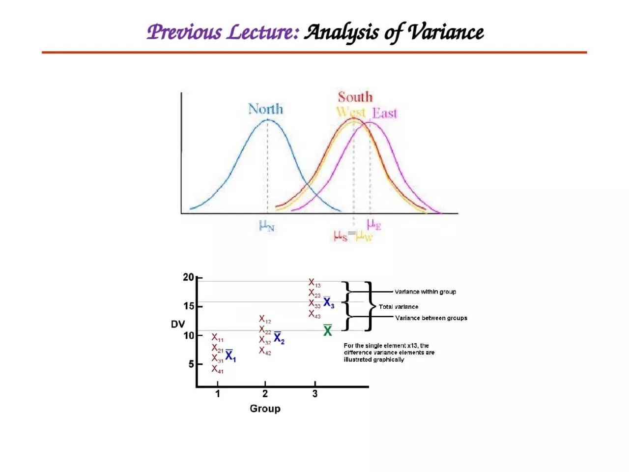
/
Previous Lecture:  Analysis of Variance Previous Lecture:  Analysis of Variance

Previous Lecture: Analysis of Variance - PowerPoint Presentation

stella
stella . @stella
Follow
0 views
Uploaded On 2024-03-13

Previous Lecture: Analysis of Variance - PPT Presentation

Categorical Data Methods This Lecture Judy Zhong PhD Outline Categorical data Definition Contingency table Example Pearsons 2 test for goodness of fit 2 test for two population proportions ID: 1047847

left test expected handed test left handed expected cell reject proportion frequency table exact contingency proportions sample females square

Share:

Link:

Embed:

Download Presentation from below link

Download Presentation The PPT/PDF document "Previous Lecture: Analysis of Variance" is the property of its rightful owner. Permission is granted to download and print the materials on this web site for personal, non-commercial use only, and to display it on your personal computer provided you do not modify the materials and that you retain all copyright notices contained in the materials. By downloading content from our website, you accept the terms of this agreement.


Presentation Transcript

1. Previous Lecture: Analysis of Variance

2. Categorical Data MethodsThis LectureJudy Zhong Ph.D.

3. OutlineCategorical dataDefinitionContingency tableExamplePearson’s 2 test for goodness of fit2 test for two population proportions (Z test to compare two proportions)2 test of independence in a contingency tableFisher’s exact test –small sample size

4. Categorical dataDefinition: refers to observations that are only classified into categories so that the data set consists of frequency counts for the categories.Example:Blood type (O, A,B,AB)A shipment of assorted nuts (walnuts, hazelnuts, and almonds) Gender (male, female)

5. Example 1. Two population ProportionsIn a random sample, 120 Females, 12 were left handed; 180 Males, 24 were left handedGenderHand PreferenceLeftRighttotalFemale 12108120Male24156180Total36264300

6. Example 2:Independent Samples classified in Several categories:The meal plan selected by 200 students is shown below:ClassStandingNumber of meals per weekTotal20/week10/weeknoneFresh.24321470Soph.22261260Junior1014630Senior14161040Total 708842200

7. Contingency TablesContingency TablesUseful in situations involving multiple population proportionsUsed to classify sample observations according to two or more characteristicsAlso called a cross-classification table.

8. Pearson’s 2 test: for two population propotions(example 1)Sample results organized in a contingency table:GenderHand PreferenceLeftRightFemale12108120Male2415618036264300120 Females, 12 were left handed180 Males, 24 were left handedsample size = n = 300:

9. 2 Test for the Difference Between Two ProportionsIf H0 is true, then the proportion of left-handed females should be the same as the proportion of left-handed malesThe two proportions above should be the same as the proportion of left-handed people overallH0: p1 = p2 (Proportion of females who are left handed is equal to the proportion of males who are left handed) H1: p1 ≠ p2 (The two proportions are not the same – Hand preference is not independent of gender)

10. The Chi-Square Test Statisticwhere: O = observed frequency in a particular cell E = expected frequency in a particular cell if H0 is true 2 for the 2 x 2 case has 1 degree of freedom(Assumed: each cell in the contingency table has expected frequency of at least 5)The Chi-square test statistic is:

11. Computing the Average ProportionHere: 120 Females, 12 were left handed180 Males, 24 were left handedi.e., the proportion of left handers overall is 0.12, that is, 12%The average proportion is:

12. Finding Expected FrequenciesTo obtain the expected frequency for left handed females, multiply the average proportion left handed (p) by the total number of femalesTo obtain the expected frequency for left handed males, multiply the average proportion left handed (p) by the total number of malesIf the two proportions are equal, then P(Left Handed | Female) = P(Left Handed | Male) = .12i.e., we would expect (.12)(120) = 14.4 females to be left handed (.12)(180) = 21.6 males to be left handed

13. Observed vs. Expected FrequenciesGenderHand PreferenceLeftRightFemaleObserved = 12Expected = 14.4Observed = 108Expected = 105.6120MaleObserved = 24Expected = 21.6Observed = 156Expected = 158.418036264300

14. GenderHand PreferenceLeftRightFemaleObserved = 12Expected = 14.4Observed = 108Expected = 105.6120MaleObserved = 24Expected = 21.6Observed = 156Expected = 158.418036264300The Chi-Square Test StatisticThe test statistic is:

15. Decision RuleDecision Rule:If 2 > 3.841, reject H0, otherwise, do not reject H0Here, 2 = 0.7576 < 2U = 3.841, so we do not reject H0 and conclude that there is not sufficient evidence that the two proportions are different at  = 0.0522U=3.8410 Reject H0Do not reject H0

16. Test for Association for RxC Contingency TablesSimilar to the 2 test for equality of more than two proportions, but extends the concept to contingency tables with r rows and c columnsH0: The two categorical variables are independent (i.e., there is no association between them)H1: The two categorical variables are dependent (i.e., there is association between them)

17. 2 Test of Independencewhere: O = observed frequency in a particular cell of the r x c table E = expected frequency in a particular cell if H0 is true 2 for the r x c case has (r-1)(c-1) degrees of freedomAssumed: 1. No cell has expected value < 12. No more than 1/5 of the cells have expected values < 5The Chi-square test statistic is:

18. Expected Cell FrequenciesExpected cell frequencies:Where: row total = sum of all frequencies in the row column total = sum of all frequencies in the column n = overall sample size

19. Decision RuleThe decision rule isIf 2 > 2U, reject H0, otherwise, do not reject H0Where 2U is from the chi-square distribution with (r – 1)(c – 1) degrees of freedom

20. ExampleThe meal plan selected by 200 students is shown below:ClassStandingNumber of meals per weekTotal20/week10/weeknoneFresh.24321470Soph.22261260Junior1014630Senior14161040Total 708842200

21. ClassStandingNumber of meals per weekTotal20/wk10/wknoneFresh.24321470Soph.22261260Junior1014630Senior14161040Total 708842200ClassStandingNumber of meals per weekTotal20/wk10/wknoneFresh.24.530.814.770Soph.21.026.412.660Junior10.513.26.330Senior14.017.68.440Total 708842200Observed:Expected cell frequencies if H0 is true:Example for one cell:Example: Expected Cell Frequencies(continued)

22. Example: The Test StatisticThe test statistic value is:(continued)2U = 12.592 for  = 0.05 from the chi-square distribution with (4 – 1)(3 – 1) = 6 degrees of freedom

23. Example: Decision and Interpretation(continued)Decision Rule:If 2 > 12.592, reject H0, otherwise, do not reject H0Here, 2 = 0.709 < 2U = 12.592, so do not reject H0 Conclusion: there is not sufficient evidence that meal plan and class standing are related at  = 0.0522U=12.5920 Reject H0Do not reject H0

24. Fisher’s exact testAn alternative test comparing two proportionscompute exact probability of the observed frequencies in the contingency tableUnder H0, it is assumed that there is no association between the row and column classifications and that the marginal totals remain fixedValid for tables with small expected cell values where the usual 2 test is not applicable.At least one cell<5The exact test and the 2 test will give similar results where the use of the 2 test is appropriate.

25. Fisher’s exact testCause of deathHigh saltLow saltTotalNon-CVD22325CVD53035Total75360Example 10.17 in Rosner (p. 402)

26. Fisher’s exact test in R> table.CVD<-matrix(c(2,23,5,30), nrow=2,byrow=T)> table.CVD [,1] [,2][1,] 2 23[2,] 5 30>fisher.test(table.CVD) Fisher's Exact Test for Count Data data: table.CVD p-value = 0.6882 alternative hypothesis: true odds ratio is not equal to 1 95 percent confidence interval: 0.04625243 3.58478157 sample estimates: odds ratio 0.527113

27. SummaryCategorical dataContingency tablePearson’s 2 test for goodness of fit2 test for two population proportions2 test of independence in a contingency tableFisher’s exact test –small sample size

28. Next Lecture: Nonparametric Methods