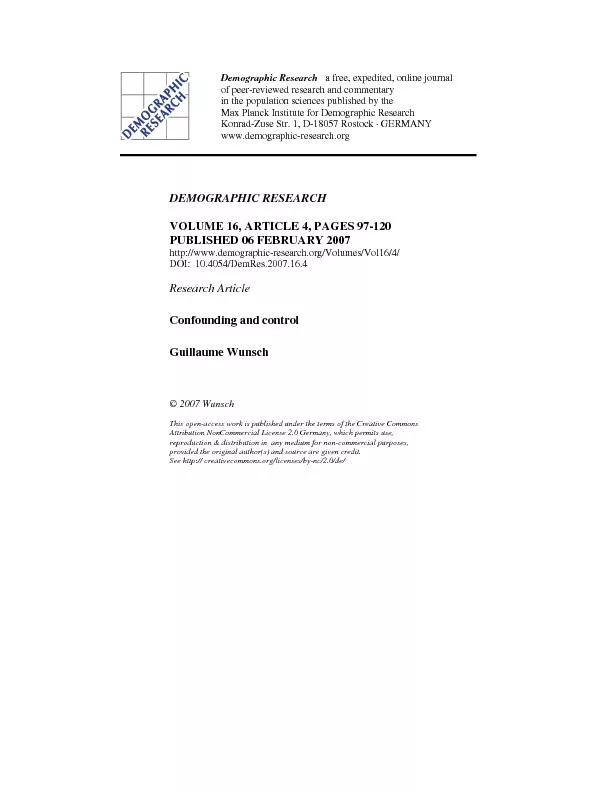
/
WunschConfounding and control  120  http://www.demographic-research.or WunschConfounding and control  120  http://www.demographic-research.or

WunschConfounding and control 120 http://www.demographic-research.or - PDF document

tatiana-dople
tatiana-dople . @tatiana-dople
Follow
424 views
Uploaded On 2016-05-22

WunschConfounding and control 120 http://www.demographic-research.or - PPT Presentation

Demographic Research Volume 16 Article 4 httpwwwdemographicresearchorg 119 Lee MJ 2005 MicroEconometrics for Policy Program and Treatment EffectsOxford Oxford University Press 262 p ID: 330149

Demographic Research: Volume Article

Share:

Link:

Embed:

Download Presentation from below link

Download Pdf The PPT/PDF document "WunschConfounding and control 120 http..." is the property of its rightful owner. Permission is granted to download and print the materials on this web site for personal, non-commercial use only, and to display it on your personal computer provided you do not modify the materials and that you retain all copyright notices contained in the materials. By downloading content from our website, you accept the terms of this agreement.


Presentation Transcript

WunschConfounding and control 120 http://www.demographic-research.org Wunsch G. (2002). The life table: a demographic overview, in: G. Wunsch, M. Mouchart, and J. Duchne (eds.). The Life Table. Modelling Survival and DeathDordrecht, Kluwer, 13-31. Wunsch G. (2006). Confounding variables, standarization, and the problem of summary indices, chapter 15 in: G. Caselli, J. Vallin, and G. Wunsch (eds.). Demography. Analysis and Synthesis. Volume 1, San Diego, Academic Press, 197-208. Wunsch H., W.T. Linde-Zwirble, and D.C. Angus (2006). Methods to adjust for bias and confounding in critical care health services research involving observational data, Journal of Critical Care, 21(1), 1-7. Demographic Research: Volume 16, Article 4 http://www.demographic-research.org 119 Lee, M-J. (2005). Micro-Econometrics for Policy, Program and Treatment EffectsOxford, Oxford University Press, 262 p.Leridon H. and L. Toulemon (1997). mographie. Approche statistique et dynamique des populations. Paris, Economica, 440 p. Mackie J. L.(1974). The Cement of the Universe: A Study of Causation. Oxford,Clarendon Press, 329 p. Mill J. S.(1889). A system of logic. London, Longmans, Green and Co., 622 p. Moffitt R. (2003). Causal analysis in population research: an economists perspective, Population and Development Review, 29(3), 448-458. Pearl J. (2000). Causality. Cambridge, Cambridge University Press, 384 p. Reichenbach H. (1956, reprinted 2000). The Direction of Time. Mineola N.Y., Dover Publications, 292 p. Robins J.M. (2001). Data, design, and background knowledge in etiologic inference, Epidemiology, 11(3), 313-320. Rothman K.J. and S. Greenland (1998). Modern Epidemiology edition, Philadelphia, Lippincott-Raven, 738 p. Rouanet H. (1985). Barouf Bombach, Bulletin de Mthodologie Sociologique, 6, 3-27. Russo F., M. Mouchart, M. Ghins, and G. Wunsch (2006). Statistical modelling and causality in the social sciences. Discussion Paper 0601, Louvain-la-Neuve, Institut de Statistique, Universit catholique de Louvain, 19 p. Schlesselman J.J. (1982). Case-Control Studies Design, Conduct, Analysis. New York, Oxford University Press, 354 p. Schlesselman J.J. (2006). The emerging case-control study: Lung cancer in relation to tobacco smoking, Preventive Medicine, in press. Schwartz D. (1994). Le jeu de la science et du hasard. Paris, Flammarion, 111 p. Smith H.L. (2003). Some thoughts on causation as it relates to demography and population studies, Population and Development Review, 29(3), 459-469. Stock J.H. and M.W. Watson (2003). Introduction to Econometrics. Boston, Addison Wesley, 696 p. Taylor R.(1966). Action and Purpose. Englewood Cliffs, NJ, Prentice-Hall., 269 p. WunschConfounding and control 118 http://www.demographic-research.org Elwood J.M. (1988). Causal Relationships in Medicine. Oxford, Oxford University Press, 332 p. Fisher R.A. (1957). Alleged dangers of cigarette smoking, British Medical Journal, II, 297-298. Fisher R.A. (1958). Lung cancer and cigarettes, Nature, 182, July 12, p. 108. Foster E.M. (2003). Propensity score matching. An illustrative analysis of dose response, Medical Care, 41(10), 1183-1192. Freedman D. (1999). From association to causation: some remarks on the history of statistics, Statistical Science, 14(3), 243-258. Gaum C. and G. Wunsch (2003). Health and Death in the Baltic States, in: I. E. Kotowska and J. Jozwiak (eds.). Population of Central and Eastern Europe. Challenges and Opportunities. Warsaw, Statistical Publishing Establishment, 301-325. rard H. (2006). Theory building in demography, chapter 129 in: G. Caselli, J. Vallin, and G. Wunsch (eds.). Demography. Analysis and Synthesis. Volume 4, San Diego, Academic Press, 647-660. Greenland S. and B. Brumback (2002). An overview of relations among causal modelling methods, International Journal of Epidemiology, 31, 1030-1037. Heckman J.J. (2005). The scientific model of causality, Sociological Methodology35(1), 1-98, with a discussion by M.E. Sobel, 99-133. Article published online 5 June 2006. Hernn M.A., S. Hernndez-Diaz, M.M. Werler, and A.A. Mitchell (2002). Causal knowledge as a prerequisite for confounding evaluation: an application to birth defects epidemiology, American Journal of Epidemiology, 155(2), 176-184. Holland P.W. and D.B. Rubin (1988). Causal inference in retrospective studies, Evaluation Review, 12(3), 203-231. Jenicek M. and R. Clroux (1982). Epidmiologie. Paris, Maloine, 454 p. Kesteloot H., S. Sans, and D. Kromhout (2006). Dynamics of cardiovascular and all-cause mortality in Western and Eastern Europe between 1970 and 2000European Heart Journal, 27(1), 107-113. Khlat M. (1994). Use of case-control methods for indirect estimation in demography, Epidemiologic Reviews, 16(1), 124-133. Demographic Research: Volume 16, Article 4 http://www.demographic-research.org 117 References Anderson S., A. Auquier, W.W. Hauck, D. Oakes, W. Vandaele, and H.I. Weisberg (1980). Statistical Methods for Comparativetudies. New York, Wiley, 289 p. Angrist J.D., G.W. Imbens, and D.B. Rubin (1996). Identification of causal effects using instrumental variables, Journal of the American Statistical Association91(434), 444-455. Angrist J.D. and A.B. Krueger (2001). Instrumental variables and the search for identification: from supply and demand to natural experiments, Journal of Economic Perspectives, 15(4), 69-85. Bartecchi C.E., T.D. MacKenzie, and R.W. Schreir (1995). The global tobacco epidemic, Scientific American, 272(5), 26-33. Best N. and P. Green (2005). Structure and uncertainty, Significance, 2(4), 177-181. Blalock H.M. (1961). Causal Inferences in Nonexperimental Research. Chapel Hill, The University of North Carolina Press, 200 p. Bollen K.A. (1989). Structural Equations with Latent Variables. Wiley, New York, 514 p. Brown S.R. and L.E. Melamed (1990). Experimental design and analysis. Newbury Park, Sage Publications, 86 p. Chalmers I. and R. Matthews (2006). What are the implications of optimism bias in clinical research?, TheLancet, 367(9509), 449-450. Coale A.J. (1973). The demographic transition reconsidered. Proceedings of the International Population Conference, Volume 1, IUSSP, Lige, 53-72. Courgeau D. (2002). flexions sur Rgression et analyse gtrique des donnes, Henry Rouanet et al., personal communication, 8 p. Courgeau D. (2003). From the macro-micro opposition to multilevel analysis in demography, chapter 2 in: D. Courgeau (ed.). Methodology and Epistemology of Multilevel Analysi., METHODOS Series N 2, Dordrecht, Kluwer, 43-91. Cox D.R. and N. Wermuth (2004). Causality: a statistical view, International Statistical Review, 72(3), 285-305. Dawid A.P. (2002).Influence diagrams for modelling and inference, International Statistical Review, 70, 161-189. WunschConfounding and control 116 http://www.demographic-research.org 5. Acknowledgments This paper is part of a research project conducted by F. Russo (University of Kent), M. Mouchart (UCLouvain), and the present author, on Causality and Statistical Modelling in the Social Sciences. It has initially been prepared as an invited paper for the seminar on Causality, Exogeneity and Explanation, Causality Study Circle Evidence Project, UCL, London, May 5, 2006. Comments and suggestions from Federica Russo and Michel Mouchart, as well as from Daniel Courgeau, Catherine Gourbin, Myriam Khlat, Godelieve Masuy-Stroobant, Laurent Toulemon, and two anonymous reviewers are gratefully acknowledged. Demographic Research: Volume 16, Article 4 http://www.demographic-research.org 115 leading to the well-known Berkson or Schwartz and Lazar formulas (see e.g. Wunsch 2002). Suppose now that a common cause such as marital status influences both mortality and migration, which is actually the case. The two variables are then associated, as Reichenbachs conjunctive forks have shown. Remember that a conjunctive fork is a causal structure where two (or more) effects have a common cause and where the effects are conditionally independent given the common cause. In this case, migration could select persons with different mortality probabilities than non-migrants and the classic formulas for computing net probabilities would be biased. As one knows in philosophy and statistics, the counterfactual approach is hardly acceptable except as a very simplified model; it would be better here to control for the common cause(s) if possible. 4. Conclusions Confounders are common causes of both treatment/exposure and of response/outcome. Some classical definitions of confounding in epidemiology or in demography, based on associations only, are incomplete as they do not consider the causal paths among the variables which lead to association. Confounding is better taken care of by randomisation at the design stage of the research. Randomisation is however unethical or impossible to achieve in many social science problems. In observational studies, conditioning on the observed confounders by stratification is recommended but the results should not be standardised if there is a strong interaction between the confounder and treatment/exposure on the outcome. If the confounder is latent, controlling for observed intervening variables or an observed surrogate confounder, or using an instrumental variable, may sometimes be possible depending on the knowledge one has concerning latent confounders. Under stronger assumptions, a fixed effects regression model can also take into account unobserved heterogeneity if longitudinal data are available. Even when the common cause is observed, it might be better in some cases but not in all to control for an intervening factor if other latent common causes are suspected or if the common cause is a remote ancestor in the causal graph. The research strategy should be based on a thorough knowledge of the field and on ones conceptual framework and causal model. In practice, as the truemodel is unknown, more than one plausible causal model will usually be tested for best fit and structural stability, reflecting the limits of our knowledge. WunschConfounding and control 114 http://www.demographic-research.org I said above that it is probably better to control for an intervening variable between the common cause and the effect, rather than for the common cause itself especially if the latter is remote from the treatment/exposure, due to the possible presence of other latent causes or the temporal reduction of influence for remote common causes. Here is however a case, borrowed from Pearl (2000) and taken up by Greenland and Brumback (2002), where this strategy would be wrong. In this model, all the variables are observed. Consider five variables U, V, Z, X, and Y, causally related as in the DAG of figure 6, and suppose we are specifically interested in the relation X causes Y. Figure 6: Common causes and intervening variable In this model, contrary to intuition, it is not sufficient to control for the intervening variable Z. Even if U and V are independent, they are associated in some strata in Z as they both cause Z. Due to the association between U and V, U is associated with Y through V and V is associated with X through U. Either V or U must be controlled for to remove the confounding. 3.9 Common causes and competing risks Finally, common causes also have an impact on the way we deal with competing risksFor example, in demography it is customary to estimate a net probability of dying at a given age in the absence of migration using a counterfactual approach. If migrants had not left the country, what would have been the probability of dying without the occurrence of migration? One usually assumes that both processes are independent, Demographic Research: Volume 16, Article 4 http://www.demographic-research.org 113 To give another example, it would be inadequate to control for the physical characteristics of the child (e.g. gestation duration) when measuring the impact of age of the mother on neonatal mortality, as these characteristics are often dependent upon this age. Physical characteristics of the child are an intermediate variable on the path from mothers age to neonatal mortality. Furthermore, controlling for a common effect of a treatment and an outcome creates a spurious association between the latter two (Hernet al.op. cit.), in addition to a possible treatment effect. This is due to the fact that two causes become correlated when one controls for their common effect (or collider). As an example, Hernconsiders two independent variables - diet and non-diet-related cancer - which become associated once we control for weight loss, a common effect of both diet and cancer. One should therefore not condition on a common effect of two (or more) variables. Another situation where it would be inappropriate to control for a covariate is the case of a conjunction of causes of the type XZ X and Z jointly cause Y. To give an example, in the case of fertility transition, Ansley Coale (1973) considers that several necessary conditions (conscious choice, advantage, effective techniques) have to be simultaneously satisfied for fertility to fall in high fertility countries. If at least one of these conditions is not satisfied, fertility will not decrease: for a decline in fertility to occur, the conjunction of the three conditions is required. A causality of conjunctions of causes has been proposed in philosophy of science by John Stuart Mill (1889) and Richard Taylor (1966), and by John Mackie (1974) with his INUS causality. Take the very simple situation where the three variables X, Z, Y, are dichotomous (presence/absence). One obtains in this case the following results Cause X Cause Z Outcome Y 1 1 1 0 1 0 1 0 0 0 0 0 Controlling for Z (conditioning on Z) means examining the relation between X and Y for Z = 1 or Z = 0. If Z = 1, one would conclude that X is a necessary and sufficient cause of Y because if X , then Y and if non X, then non Y. On the contrary, if Z = 0, one would conclude that X is not a cause of Y because Y = 0 for both X = 0 and X = 1. The general conclusion would be the existence of an interaction effect between X and Z as the influence of X on Y varies according to the values of Z. Actually, this would be a misspecified model; in reality, the interaction between both causes is so strong that the additive effects of X and of Z on Y disappear in favour of the sole conjunction XZ influencing Y. WunschConfounding and control 112 http://www.demographic-research.org If longitudinal data are available, we can control for unobserved heterogeneity due to unknown omitted variables using a time and/or entity fixed effects regression modelThis approach assumes that omitted variables are constant over time but vary among entities (observation units) while others are constant across entities but vary over time (Stock and Watson op. cit.). If these assumptions do not hold, the surrogate and IV approaches remain valuable methods of control if we have some knowledge concerning the latent confounder(s). Ones conceptual framework, based on background knowledge, formal theory, informal evidence, and research hypotheses, should take into account for this purpose all known observed latent variables relevant for the problem at hand (Moffitt 2003, Grard 2006). Even if SES is observed in the model of figure 2, it would still be advisable to control for A instead of the common cause SES if we want to measure the impact of smoking on cancer. SES might not be the only common cause of T and A, as pointed out in the previous paragraph. For example, smoking and occupation are gender-dependent; gender would also be a common cause. To give another example, an unknown gene G may make some smokers and asbestos inhalers more susceptible to cancer; the effects of smoking and asbestos exposure would then be associated through the common genotype. The common cause might also be too remote from the causal relations studied. For example, one could argue that ones SES is dependent upon oneparents SES and control for the latter. However, the more remote, the less influence the common cause probably has on the variables downstream in the model. I would therefore usually recommend controlling for more proximate intervening variables on the path from a common cause to the outcome than on the common cause itself if the latter is much further upstream in the causal graph, especially in the social sciences where multiple latent common causes are probably the norm. Note that in this case one falls back on the classic definition of a confounder as a variable associated with the treatment/exposure (through the presence of a common ancestor) and having an impact on the outcome. 3.8 or not to control? Controlling for a variable that is not a confounder can be harmful. In the model of figure 3, A should not be controlled for when studying the total impact (direct and indirect) of T on C, as A is not a confounder but an intermediate variable in the indirect path going from T to C through A, in addition to the direct path T to C. Controlling for A would only be justified if one wished to evaluate solely the direct effect of T on C. Do not confuse with a fixed effects ANOVA model where levels are deliberately set by the researcher. Demographic Research: Volume 16, Article 4 http://www.demographic-research.org 111 estimates of the causal effects of health inputs on health outcomes. The sex composition of the first two births in families with at least two children has been used as an IV to estimate the effect of additional children on parents' labour supply. Ways to partially test these conditions can be found in the econometric literature. Furthermore, procedures robust to the presence of weak instruments are being developed. Note the resemblance and the difference between the surrogate and the instrumental variable approaches (figure 5). In the surrogate case we use a proxy of SES while the IV approach uses a proxy of T. One assumes in the IV approach that the covariance between IV and SES is nil while the covariance between IV and T is strong. In the surrogate approach, one assumes on the contrary that the covariance between K and SES is high. More precisely, one has the following independence assumptions. For the approach: IV SES IV The second condition stems from the fact that the only path from IV to C must be through T (Angrist and Krueger 2001); this last constraint is often overlooked in econometric textbooks. For the surrogate approach : T, C SES This condition states that the only path from K to T and C is through SES. On the other hand, C is not independent of T given SES, as one postulates that smoking is a cause of cancer. Figure 5: Surrogates and instrumental variables SES C WunschConfounding and control 110 http://www.demographic-research.org 3.6 To control … ? When should we control for a background variable and when should we not control for this variable, when examining the impact of a treatment/exposure on an outcome in an observational (i.e. non-experimental) study? In other words, is this variable a confounder or not? If the background variable is a common cause of both treatment/exposure and outcome, it should be controlled for. Let us go back to the previous figures 2 to 4. In figure 2, SES has to be controlled for in this model if one wants to estimate the impact of smoking on cancer of the respiratory system in the absence of confounding, taking into account the definition of a confounder given in the previous section. SES is a common cause of smoking (exposure) and of cancer (outcome) via A, as SES is in the DAG a parent of both tabacism and asbestos exposure. In this case, conditional on SES, the variables tabacism and asbestos exposure should become independent and the association between them should disappear; if not, a latent common cause is most probably present. To give another example, in the model of figure 4, if one is interested in the relation between T and C, A should be controlled for as A is a common cause of both the exposure T and the outcome C. 3.7 Controlling for a latent confounder Suppose now that SES is itself latent, i.e. unobserved. We could also block the impact of SES by controlling for A on the path from SES to C (the outcome), as A is observed, or by conditioning on an observed intermediate variable between SES and T (the treatment/exposure). In the absence of such observed intervening variables, we could also control for any observed variable K (e.g. income) deemed to be highly correlated with the latent variable SES on the basis of our background knowledge, using K as a surrogate for SES (Hernet al. 2002). The correlation between K and SES can be causal or not; the observed K is then used in place of the unobserved SES. To give some examples from the literature, sex can be used as a proxy for gender, educational level for income, country of origin for ethnicity, infant mortality rate for income distribution, etc., if it is deemed that there is a strong correlation between the proxy and the variable of interest. We could also use an instrumental variable (IV) approach (Stock and Watson 2003), choosing an IV such that the correlation or covariance between the IV and the putative cause is strong (instrument relevance) while the correlation or covariance between the IV and the latent confounder is nil (instrument exogeneity). For example, prices of health inputs are the most common instrumental variable for identifying Demographic Research: Volume 16, Article 4 http://www.demographic-research.org 109 or the outcome is sufficient for controlling for the confounder. For example, taking the Treatment population structure as standard, one would obtain the following global rates: (30 x 0.60 + 10 x 0.20)/40 = 0.50 for the Treatment group (30 x 0.70 + 10 x 0.30)/40 = 0.60 for the No treatment group This time, the combined standardized rate does lead to the same conclusion as the analysis by gender: the recovery rate (both genders) is lower in the Treatment group than in the No treatment group. Furthermore, no interaction is present here as the absolute difference is the same for males and for females, i.e. 10 per cent. In this situation, the same global result would be obtained whatever the standard population. The treatment should therefore be discontinued. However, standardisation breaks down when there are interaction effects (see Wunsch 2006, for a general discussion). In the case of strong interaction, no linear combination of rates can represent the true results because more than one indicator per group is required in this situation. If this were the case in the present example, no averaging of the results by gender could lead to a satisfactory global indicator. For example, consider the situation where the recovery rates would be 0.60 (males) and 0.40 (females) in the Treatment group, and respectively 0.70 and 0.30 in the No treatment group. According to the choice of the arbitrary standard population, one could say that the global recovery rate in the Treatment group is lower, equal, or higher than in the No treatment group, a conclusion which is not very informative! No sole measure can tell us that the recovery rate for males is lower in the Treatment group compared to the No treatment group while the converse is true for females (i.e. strong interaction between treatment and gender). 3.5 Multilevel modelling Suppose now that the hospital where the patients are treated is associated both with treatment and recovery. In addition to taking a sample of patients per hospital, one can also draw a sample of hospitals and take into account both the treatment effect at the individual level and the hospital effect at the contextual level, using a multilevel model. Daniel Courgeau has shown that this type of model elegantly resolves Simpsonparadox; it can furthermore include interaction terms between the individual and contextual variables (Courgeau 2002, Courgeau 2003). The approach lies however outside the scope of this paper. WunschConfounding and control 108 http://www.demographic-research.org Table 1: Treatment, recovery, and gender Both genders Recovery No recovery Total Recovery rate Treatment 20 20 40 .50 No treatment 16 24 40 .40 Total 36 44 80 Males Treatment 18 12 30 .60 No treatment 7 3 10 .70 Total 25 15 40 Females Treatment 2 8 10 .20 No treatment 9 21 30 .30 Total 11 29 40 Source: Pearl, 2000 It is easy to show why the treatment seems to have an effect in the general population while this conclusion does not hold in each gender category. The combined recovery rates in the Treatment and No treatment groups can be written as follows: (30 x 0.60 + 10 x 0.20)/40 = 0.50 for the Treatment group (10 x 0.70 + 30 x 0.30)/40 = 0.40 for the No treatment group In the Treatment group, there is a higher proportion of males than females, and males have a higher recovery rate than females. The opposite is true in the No treatment group. Males thus opt for treatment more than females and they have a higher recovery rate because, for example, their compliance might be higher. Gender is therefore a confounding factor, as the two sub-populations differ by gender structure i.e., gender has an impact on opting for treatment or not) and gender influences the recovery rate. To put it briefly, unconditional independence does not imply conditional independence and vice versa. 3.4 Standardisation In order to obtain an unbiased global indicator, gender combined, standardisation is often recommended: the rates by gender are applied to a same arbitrary standard population structure. This procedure actually blocks in this example the causal link from gender to treatment use. Blocking the link from the confounder to either the cause Demographic Research: Volume 16, Article 4 http://www.demographic-research.org 107 and Angus 2006). Several controls are usually matched to each case on possible observed confounders such as age or gender. Matching does not ensure however that cases and controls are alike on latent variables. All possible sources of confounding bias are not avoided, contrary to ex ante randomisation in prospective studies. In addition, the comparison between cases and controls can be done in terms of odds ratios but not of relative risks, as the population exposed to risk is unknown. Finally, as in all retrospective studies, only persons alive are included in the study and they may differ from those who have died. On the other hand, retrospective case-control studies are much less expensive and time-consuming to carry out than prospective randomised trials. Case-control studies are too rarely conducted in the social sciences and in demography in particular. 3.3 Controlling ex post in non-experimental studies In non-experimental (observational) studies, prospective or retrospective, the two major ex post approaches for controlling for confounders are stratification for categorical variables and statistical adjustment for numerical variables. This distinction is not clear-cut however, as statistical adjustment can be applied to categorical variables using . logit regression, and a numerical variable can always be categorised age can be transformed into age groups for example. These approaches can take into account observed confounders but are hardly able to control for latent ones. To keep this paper succinct, the stratification approach will mainly be developed here; for other methods, see . Wunsch, Linde-Zwirble and Angus (2006)In an observational study, stratification implies conditioning on the confounding variable(s). This approach will be considered in the case of the well-known Simpson’s paradox; the example is taken from Pearl (2000, pp. 174-175). In a population suffering from a disease, one sub-population follows a treatment and the other does not. The treatment increases the recovery rate when both genders are combined. On the other hand, when gender is taken into account (controlled for), the drug decreases the recovery rate both for males and for females, thus the paradox. Table 1 distributes the population by treatment, recovery, and gender. WunschConfounding and control 106 http://www.demographic-research.org 3.2 Treatment selection in non-experimental studies In prospective studies with non-random allocation, there is always a risk that the characteristic on which the allocation is done is associated with the outcome, inducing unobserved heterogeneity so that the treatment effect cannot be distinguished from the selection effect, though matching (in particular propensity score matching) can to some extent reduce the problem (Lee 2005). A propensity score is the predicted probability of receiving the treatment/being exposed, taking into account observed covariates. For the two-group case, one can run a logistic regression with the dependent variable Y = 1 if treated and Y = 0 if not, with appropriate observed conditioning variables One then obtains the probability score or predicted probability or odds of treatment (or non-treatment) selection. Each participant in the treatment is then matched with one or more non-participants on the basis of their propensity score. For a practical example, see e.g. Foster (2003). A major disadvantage of this method, as Heckman (2005) has shown, is that it assumes that the marginal person receiving treatment is the same as the average person. On the contrary, the method of control functions (see Heckman op. cit.) allows the marginal treatment effect to be different from the average treatment effect. Another approach at the design stage is to take into account an instrumental variable (IV), the IV being highly correlated with the treatment but independent of the suspected latent confounder - or error term - possibly influencing both treatment and outcome. For example, prices of cigarettes might be taken as an IV when studying the relation between tabacism of the mother and child birthweight. Price should affect the likelihood of being a smoker but there is no reason to believe it affects birthweight through another path (this and several other examples are discussed in Moffitt 2003). A two-stage procedure yields in this case a non-biased estimation the IV has been well chosen, i.e. if it satisfies the two criteria pointed out above (Angrist, Imbens and Rubin 1996). In the analysis, the treatment influenced by the latent confounder is replaced by an IV independent of the latter (see the paragraph on latent confounders below). Actually, it is hardly possible to check the independence assumption between IV and error term, as the latter is latent, except on the basis of background knowledge. In retrospective studies, ex ante randomisation is not possible, as the subjects either have or have not been subjected to the treatment and to the outcome (Holland and Rubin 1988). A case-control study on the relation between smoking and lung cancer would compare the past smoking history of persons alive with lung cancer, i.e. those having experienced the outcome, to a control group of ex post randomly selected persons without lung cancer (Khlat 1994, and the other articles in the special issue of this journal on case-control studies). The method is however subject to information bias, i.e. recall lapses which differ among cases and controls (Wunsch, Linde-Zwirble A somewhat similar approach had been proposed by H.M. Blalock (1961). Demographic Research: Volume 16, Article 4 http://www.demographic-research.org 105 optimism bias i.e., unrealistic expectations, for both patients and clinicians, of the likely benefits of new treatments in randomised trials (Chalmers and Matthews 2006). Randomisation ensures to a high extent that both groups differ only by the fact that one receives the treatment (the cause) and the other not. The causal relation between treatment and outcome (e.g. recovery) is not affected by a confounder - observed or unobserved - due to the fact that the two groups are similar in all respects except treatment/no treatment. In particular there is no selection bias. The absence of selection bias does not mean however that the target group is homogeneous as concerns treatment effect; the group may contain sub-groups which vary widely in response to the treatment (Schwartz 1994). For example, in the target group females may react better to the treatment than males, younger persons than older ones, etc. If known, these factors can be taken into account in the experimental design by stratified randomisation (factorial design). For example, if one suspects that the treatment effect may vary by gender, one will enter both treatment and gender in the same experiment. An ANOVA will then yield the separate and interactive effects of treatment and gender. However, unobserved heterogeneity may remain due to the presence of unknown latent factors of e.g. genetic origin. A randomised experiment furthermore does not show how the treatment will be used in the real world: who will desire the treatment and who will opt out, what will be his or her compliance, what will be the unwanted indirect effects of the treatment (Smith 2003). For example, the pill is a highly effective method of contraception under laboratory conditions (theoretical effectiveness) but in practice (use-effectiveness) it may nevertheless lead to many unwanted pregnancies if it is carelessly used. Though quite common in clinical studies, randomisation can however be unethical or impossible to conduct. For moral reasons, one may not randomly allocate subjects, for example, between a smoking group and a non-smoking group, or between receiving a treatment A and no treatment at all if an alternative treatment is already available. Presently, in clinical trials, the alternative treatment must be given to the control group instead of a placebo. Furthermore, subjects are now required to give their consent in order to participate in the study. To give another example, allocating subjects to different income groups in order to examine the causal relation between income and fertility would not be unethical but impractical. For these reasons, randomisation is very often impossible in the social sciences. It is however practised in educational studies, among others, in order to compare e.g. the performance of students following a physics course based on lectures to a physics course based on project development. In addition, to avoid course-teacher interaction, teachers are usually rotated between both types of courses. Finally, all prospective studies - randomized or not - are affected by loss to follow-up. If those who drop out of the study differ from those who stay, the relation between treatment and outcome may become biased. WunschConfounding and control 104 http://www.demographic-research.org cause of T and C; A does not therefore confound the relation between T and C. The confounder can be either latent (i.e. unobserved) or observed. From the point of view of controlling for the confounder, the two cases are obviously quite different (see Cox and Wermuth 2004). This definition avoids taking an intervening (intermediate) variable between the putative cause and the outcome such as in figure 3 as a confounder, even though it is associated with the putative cause (as the latter has a causal influence on the former) and it has an impact on the outcome. Many definitions given in epidemiology or demography are not adequate in this respect. As one can presume, the possible confounder should not be affected by treatment/exposure (Schlesselman 1982). Finally, how does conditional independence relate to confounding and control? Using the so-called d-separation criteria, it is possible in causal graphs to check for conditional independence (Pearl 2000, Robins 2001). Considering three disjoint sets of variables X, Y, and Z, which are represented as nodes in a DAG, following Pearl a path between X and Y is d-separated or blocked by a set of nodes Z if and only if the path contains a chain x z y or a fork x y such that the middle node z is in Z, or the path contains an inverted fork or collider x m y such that the middle node m is not in Z and such that no descendant of m is in Z. Our definition of confounding relates to the fork x z y. In this case, z should be controlled in order to assess the relation between x and y, but what happens if we control for z or for m in the case of a chain or a collider? These questions are examined in the following section, more particularly in sub-sections 3.6 to 3.8. 3. Control 3.1 Controlling ex ante: randomisation in prospective studies If possible confounding is suspected, it should ideally be taken into account at the design stage of the study (see e.g. Rothman and Greenland 1998, Lee 2005). The best way to avoid confounding bias in a prospective study is ex ante randomisation, i.e. a random allocation of subjects between the treatment and the control groups. In the simplest case, the first group receives the treatment and the second a placeboMoreover, in view of avoiding investigator bias, the procedure should be kept secret from the investigator. Actually, double-blind experiments are often conducted in clinical epidemiology, both the clinician and the subject ignoring whether the latter is put into the treatment group or into the control group. Double-blind studies avoid For an introduction to more complex experimental designs, see Brown and Melamed (1990). Demographic Research: Volume 16, Article 4 http://www.demographic-research.org 103 TAC The second case is represented by figure 4, A being this time a common cause of T and C. ATC This distinction leads to a more precise definition of a confounder: a confounding variable or confounder is a variable which is a common cause of both the putative cause and its outcome (Bollen1989, Pearl 2000). For example, A confounds the relation between T and C in figure 4 because it is in this model a common cause of both T and C. For the same reason, SES is a confounder in figure 2, as it is a common cause of both T and C (the latter via A). In figure 3, the intervening variable A is not a common WunschConfounding and control 102 http://www.demographic-research.org Coming back to the question why are smoking and asbestos exposure associated?, one knows in demography and in epidemiology that both smoking and asbestos exposure are dependent upon ones socio-economic status (SES): those with a lower SES tend more to smoke and work in unhealthy environments than those with a higher SES. The causal graph can therefore be drawn as in figure 2, where A represents exposure to asbestos, T tabacism, and C cancer incidence. Figure 2: Socio-economic status (SES), tabacism (T), asbestos exposure (A), and cancer of the respiratory system (C) SES This graph shows that tabacism and asbestos exposure are in fact not independent from one another as they are both related to ones SES, i.e. they have a common cause. This association or correlation is represented here by a non-directed edge between A and T. Note that SES is also a common cause of T and C as it has an impact on cancer through the intervening or intermediate variable asbestos exposure A, a variable on the path from SES to C. An association between two variables such as smoking and asbestos exposure could however also be due to a causal relation between them. T could be a cause of A or vice-versa. The first situation, T causes A, is represented in figure 3; A is an intervening variable between T and C in this case. Some authors represent an association between two variables by a double-headed arrow. This representation is however more suited to feedback effects in nonrecursive models. Demographic Research: Volume 16, Article 4 http://www.demographic-research.org 101 2.2 A confounder as a common cause Condition 1 needs to be clarified however. Why are smoking and asbestos exposure associated? Hans Reichenbach (1956) was one of the first, if not the first, in philosophy to point out that simultaneous correlated events must have a prior common cause: If improbable coincidence has occurred, there must exist a common cause (p.157). At around the same time, statisticians were also aware that a correlation between two variables could be due to a common cause. Considering once again the correlation between smoking and lung cancer, suppose that ones unknown genotype (G) would influence both smoking behaviour or tabacism (T) and the susceptibility to lung cancer (C). This explanation was proposed by the statistician R.A. Fisher when he was scientific consultant to the Tobacco Manufacturers Standing Committee in the late 1950s (Fisher 1957). Thus, without any direct causation being involved, both characteristics might be largely influenced by a common cause, in this case the individual genotype (Fisher 1958). The corresponding causal graph is presented in figure 1 with possibly no causal link at all between T and C. Fishers suggestion was ultimately disproved but it did show that proving the relation between lung cancer and cigarette smoking required not only sound epidemiological evidence, but also replication in different studies, experimental evidence from animal studies, and a plausible biological mechanism linking smoking to lung cancer. Figure 1: Tabacism and cancer associated by genotype GenotypeTabacismCancer WunschConfounding and control 100 http://www.demographic-research.org Angus (2006). For the issue of conditioning by intervention and the use of influence diagrams, see Dawid (2002). 2. Confounding 2.1 What is confounding? In epidemiology and in demography, when one examines the impact of a treatment or exposure on a response or outcome, a confounding variable or confounder is often defined as a variable associated both with the putative cause and with its effect (see e.g. Jenicek and Clroux 1982, Elwood 1988). Sometimes the definition is more precise, such as in Anderson et al. (1980) or Leridon and Toulemon (1997). According to these authors, a variable, or background factor, is a confounder whenever two conditions simultaneously hold: 1. The risk groups differ on this variable; 2. The variable itself influences the outcome. To condition one, some authors furthermore add that the background factor should not be a consequence of the putative cause (Schlesselman 1982). For example, if we examine the impact of cigarette smoking on the incidence of cancer of the respiratory system, a variable such as exposure to asbestos dust confounds the relation between smoking and this type of cancer. Exposure to asbestos dust and smoking are associated, i.e. there are proportionally more persons exposed to asbestos in the smoking group than in the non-smoking group. Condition 1 is therefore satisfied. In addition, inhaling asbestos dust is a strong cause of cancer of the pleura; condition 2 is thus also satisfied. Cancer is the outcome variable in this example, smoking a potential cause, and exposure to asbestos a confounder. Vice-versa if one were to examine the impact of asbestos exposure on the incidence of cancer of the respiratory system, smoking this time would be the confounding factor, as it is associated with asbestos exposure and is a cause of lung cancer. This simplified example is developed in Russo et al. (2006); an actual study would also consider the synergistic effects between smoking and asbestos exposure, time-lags and duration of exposure, and other causal factors and paths. Contrary to tabacism, there is of course no addiction to asbestos exposure but the duration of exposure must be considered. Demographic Research: Volume 16, Article 4 http://www.demographic-research.org 99 common cause. The example of the drop in atmospheric pressure causing both a storm and a barometer dip is well-known. Simpsons paradox too is a classic example of confounding (Rouanet 1985). Simpsons paradox refers to the reversal of the direction of an association when data from several groups are combined to form a single group. In demography, one knows since the end of the 19 century that the differences in mortality between countries or regions might be due to their differential age structure only. The latter confounds in this case the actual geographical mortality pattern that one would observe in the absence of confounders. To give other examples in the field of demography, poverty might confound the relationship between alcohol consumption and mortality. Family background characteristics may confound the relationship between maternal age and child development. Education is a potential confounder of the relationship between obesity and mortality, as obesity prevalence varies significantly across groups by education level, in the U.S. for example, and mortality differentials by education level are observed overall. In this case however, one could also argue that obesity might lead to poorer results in school, leading to a two-way causation between both variables. Nonrecursive systems (reciprocal causation or feedback loops) will however not be discussed in this paper. In all these cases, the recommended remedy is to control for the confounding factor, e.g. the atmospheric pressure in the weather example or the age structure in the demographic case. This paper will deal both with the issues of confounding and of control, as the definition of a confounding factor is far from universal and there exist different methodological approaches, ex ante and ex post, for controlling for a confounding factor. As a visual representation of conditional independence structures, I will use directed acyclic graphs (DAG) where nodes represent variables and directed edges (single-headed arrows) the possible impact of the variable at the base of the edge on the variable at the head of the edge. Graphical models of this type, and the related conditional independence assumptions, are discussed in e.g. Best and Green (2005). It should be pointed out too, following Pearl (2000) and Dawid (2002), that one should distinguish between conditioning by observation and by intervention. To be succinct, the section on control will only consider the conditioning approach on observational data, though one may intervene in the population field by changing public policies. Note that many demographic characteristics such as age, sex or ethnicity can hardly be manipulated though they are well-known risk factors of e.g. AIDS. Causes understood as risk factors are not restricted to variables which can be manipulated. For example, we know that older men have a higher risk of developing prostate cancer than younger men. We cannot manipulate age of course but we can develop preventive measures which can lead and have led to a reduction in mortality due to this cancer. Other methods of control are briefly presented and discussed in Wunsch, Linde-Zwirble and WunschConfounding and control 98 http://www.demographic-research.org 1. Introduction In a recent paper on trends in cardiovascular diseases (CVD) in Europe (Kesteloot, Sans and Kromhout 2006), the authors attribute the dramatic current decline in mortality in the Baltic States to a change in dietary habits, i.e. the greater consumption of vegetable oil for cooking and the progressive replacement of butter by low-fat margarine. Though nutrition does indeed play a significant role on the incidence of CVD, one may also postulate (Gaumé and Wunsch 2003) in the case of the Baltic States that the tremendous change from a communist regime to a liberal one has led to systemic repercussions in the whole society which have brought about both modifications in cardiovascular mortality (through major fluctuations in stressful events), in economic conditions, and in behaviours including nutrition. Societal transformations and contextual changes in the economic, social (including public health), and political spheres would therefore be a confounder masking the true relation between changes in mortality patterns and in nutritional ones. To put it simply, correlation of time series does not imply causation. To take another example that will be discussed later in this paper, medical reports in the 1920s already pointed out the suspected links between tobacco and cancers, and a 1938 article in the journal Science suggested that heavy smokers had a shorter life expectancy than nonsmokers. In 1939, F.H. Müller also published a paper in German on the relationship between smoking and lung cancer (Bartecchi, MacKenzie and Schreier 1995, Freedman, 1999). Though one now knows that smoking is bad for one’s health, actually it is only in the early 1950s that two influential case-control studies, by Wynder and Graham in the U.S. and by Doll and Hill in the U.K., showed that cigarette smoking was a plausible cause of lung cancer. The relationship was confirmed by two prospective studies conducted by Doll and Hill in the U.K. and by Hammond and Horn in the U.S. (Schlesselman 2006). Even then the relationship between lung cancer and cigarette smoking was hotly disputed by a respectable scientist such as R.A. Fisher who argued as above that correlation was not causation. When is a correlation causal and when is it the result of confounding? This is the issue tackled here, by recalling some well-known and lesser-known facts. On the other hand, I will not be concerned with the diagnosis of causation and the assessment of evidence (see Elwood 1988, chapter 8). Confounding is not a new issue. In philosophy of science, Hans Reichenbach (1956) already showed the presence of screening-off effects between two variables in conjunctive forks, due to the existence of a common cause. For Reichenbach, a conjunctive fork is a causal structure where two (or more) effects have a common cause and where the effects are conditionally independent given the common cause: the association between the effects disappears when one controls for or conditions on the Demographic Research: Volume 16, Article 4 research article http://www.demographic-research.org 97 Confounding and control Guillaume Wunsch Abstract This paper deals both with the issues of confounding and of control, as the definition of a confounding factor is far from universal and there exist different methodological approaches, ex ante and ex post, for controlling for a confounding factor. In the first section the paper compares some definitions of a confounder given in the demographic and epidemiological literature with the definition of a confounder as a common cause of both treatment/exposure and response/outcome. In the second section, the paper examines confounder control from the data collection viewpoint and recalls the stratification approach for ex post control. The paper finally raises the issue of controlling for a common cause or for intervening variables, focusing in particular on latent confounders. Institute of Demography, University of Louvain (UCLouvain), Louvain-la-Neuve, Belgium. E-mail: wunsch@demo.ucl.ac.be Table of Contents 1 Introduction 98 2 Confounding 100 2.1 What is confounding? 100 2.2 A confounder as a common cause 101 3 Control 104 3.1 Controlling ex ante: randomisation in prospective studies 104 3.2 Treatment selection in non-experimental studies 106 3.3 Controlling ex post in non-experimental studies 107 3.4 Standardisation 108 3.5 Multilevel modelling 109 3.6 To control ? 110 3.7 Controlling for a latent confounder 110 3.8 or not to control? 112 3.9 Common causes and competing risks 114 4 Conclusions 115 5 Acknowledgments 116 References 117 Demographic Research a free, expedited, online journal of peer-reviewed research and commentary in the population sciences published by the Max Planck Institute for Demographic Research Konrad-Zuse Str. 1, D-18057 Rostock · GERMANY www.demographic-research.org DEMOGRAPHIC RESEARCH VOLUME 16, ARTICLE 4, PAGES 97-120 http://www.demographic-research.org/Volumes/Vol16/4/ DOI: 10.4054/DemRes.2007.16.4Research Article © 2007 Wunsch This open-access work is published under the terms of the Creative Commons Attribution NonCommercial License 2.0 Germany, which permits use, reproduction & distribution in any medium for non-commercial purposes, provided the original author(s) and source are given credit. See http:// creativecommons.org/licenses/by-nc/2.0/de/