PDF-13th World Conference on Earthquake Engineering

Author : tawny-fly | Published Date : 2017-08-16

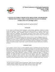
C Canada August 16 2004 Paper No 2 A STUDY ON ENERGY DISSIPATING BEHAVIORS AND RESPONSE PREDICTION OF RC STRUCTURES WITH VISCOUS DAMPERS SUBJECTED TO EARTHQUAKES

Presentation Embed Code

<iframe width="560" height="315" src="https://www.docslides.com/embed/79037" frameborder="0" allowfullscreen></iframe>

Download Presentation

Download Presentation The PPT/PDF document "13th World Conference on Earthquake Engi..." is the property of its rightful owner. Permission is granted to download and print the materials on this website for personal, non-commercial use only, and to display it on your personal computer provided you do not modify the materials and that you retain all copyright notices contained in the materials. By downloading content from our website, you accept the terms of this agreement.

13th World Conference on Earthquake Engineering: Transcript

Download Document

Here is the link to download the presentation.
"13th World Conference on Earthquake Engineering"The content belongs to its owner. You may download and print it for personal use, without modification, and keep all copyright notices. By downloading, you agree to these terms.