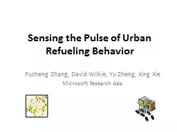
/
Sensing the Pulse of Urban Sensing the Pulse of Urban

Sensing the Pulse of Urban - PowerPoint Presentation

trish-goza
trish-goza . @trish-goza
Follow
345 views
Uploaded On 2019-03-19

Sensing the Pulse of Urban - PPT Presentation

Refueling Behavior Fuzheng Zhang David Wilkie Yu Zheng Xing Xie Microsoft Research Asia Questions How many liters of gas have been consumed in the past 1 hour in NYC Which gas station in 3 miles has the shortest queue ID: 758052

time duration station gas duration time gas station refueling temporal expected average features number waiting learning distance std spatial stations queue minute

Share:

Link:

Embed:

Download Presentation from below link

Download Presentation The PPT/PDF document "Sensing the Pulse of Urban" is the property of its rightful owner. Permission is granted to download and print the materials on this web site for personal, non-commercial use only, and to display it on your personal computer provided you do not modify the materials and that you retain all copyright notices contained in the materials. By downloading content from our website, you accept the terms of this agreement.


Presentation Transcript

Slide1

Sensing the Pulse of Urban Refueling Behavior

Fuzheng Zhang, David Wilkie, Yu Zheng, Xing XieMicrosoft Research AsiaSlide2

Questions

How many liters of gas have been consumed in the past 1 hour in NYC?Which gas station in 3 miles has the shortest queue?Slide3

Goal

Use GPS-equipped taxicabs as a sensor to capture both Waiting time at a gas station City-wide petrol consumption

City-scale Gas consumption

Waiting

time of taxis in a gas station Slide4

Motivation

Gas stations are owned by competing organizations Do not want to make data available to competitorsThere is a cost but no benefit for themBenefitsGas station recommendationSupport the planning and operation of gas stations

Monitoring real-time city-scale energy consumption Slide5

Methodology Overview

1. Refueling event detection in a gas station

2. Waiting time inference across different stations

3. Estimation number of vehicles in a station

Queue theory

Tensor Decomposition

Spatio

-temporal clustering and classificationSlide6

Refueling Event Detection

Candidate ExtractionFilteringTrain a classification model with human labeled dataSpatial-Temporal features: EncompassmentGas Station Distance

. Distance To Road.

Minimum Bounding Box Ratio

.

Duration

.

POI

features including:

Neighbor Count

.

Distance To POI. Slide7

Expected Duration Learning

Infer the waiting time of each gas stationData sparsity problemModel the data as a tensorTensor decomposition with contextsSlide8

Expected Duration Learning

Tensor decompositionApproximate a tensor with the multiplication of three (low-rank) matrices and a core tensorHigh order singular value decomposition (HOSVD)Find out the three attributes’ latent connections in subspaces through what we have already observe


Neglecting other context of a station!Slide9

Expected Duration Learning

The context of a stationPOI feature

Traffic feature

Area feature


Stations with similar contextual features tend to have

a similar

durationSlide10

Expected Duration Learning

Tensor decomposition with Context<

,

> formulate a matrix

B

B

reduces the uncertainty

issues

is the parameter modeling the influence of contextual feature


L.

Baltrunas

, B. Ludwig, and F. Ricci, “Matrix Factorization Techniques for Context Aware,” pp. 301–304.Slide11

Expected Duration Learning

Tensor decomposition with contextsAn item’s contextual features are often modeled in collaborative filtering to help reduce uncertainty

issuesContext features: <

,

>

is the parameter

modeling the influence of contextual

feature


L.

Baltrunas

, B. Ludwig, and F. Ricci, “Matrix Factorization Techniques for Context Aware,” pp. 301–304.Slide12

Arrival Rate Calculation

Infer the number of vehicles in a station according to the stay duration of a taxiInsightsStay duration = waiting time + refueling time

Drivers will always choose the shortest queueEach queue could have the same length

Model each gas station as a queue system

Arrival in

a queue

is Poisson

process

Service

time satisfies exponential distribution

 Slide13

Arrival Rate Calculation

is the equilibrium system time including both the waiting time and service time

We can obtain

from the data

is the number of servers

service time (time for refueling)

The goal is to estimate the arrival rate

given

,

, and

 Slide14

Arrival Rate Calculation

Estimate I

nsight: the shortest duration of refueling events corresponds to the service time

Calculate the average time of the top

500

quickest refueling behavior

Estimate

(the number of servers)

It should be available in the real world

We use satellite maps to estimate the size of station

 number of queues

Street view images: number of pump and number of nozzles in a queue

)

 Slide15

Evaluation

RawTrajectories

Total Taxi Count

32476

Duration

54 day

Ave Distance By Day

226.76 km

Ave Sampling Interval

1.02 minute

Detected

REs

Total Count

638,645

Average Temporal Interval

1.84 day

Average Distance Interval

378.61 km

Average Duration

10.53 minute

Minimal Duration

3.74 minute

Maximal Duration

42.72 minuteSlide16

Evaluation

Manually labeled datasetsDS1: 250 real refueling events (200 for training and 50 for testing)DS2: 2,000 candidates with noisy (True/False)In the field studyDS3:Two real

users: GPS trajectories + Credit card transactions in gas station

33 records in total

DS4:

Sent students to two stations to observe the queues

Oct.17 to Nov.15 in 2012,

5:00pm

to

6:00pm.Slide17

Results

Refueling event detectionCandidate detectionFiltering

Temporal Distance (minute)

DS1

DS3

Mean

Std.

Mean

Std.

1.07

0.41

0.52

0.27

1.25

0.53

0.71

0.22

+

2.32

0.46

1.23

0.24

Temporal Distance (minute)

DS1

DS3

Mean

Std.

Mean

Std.

1.07

0.41

0.52

0.27

1.25

0.53

0.71

0.22

2.32

0.46

1.23

0.24


Features

Precision

Recall

DS2

Non-Filtering

0.464

1.0

Spatial

0.623

0.73

Spatial+Temporal

0.891

0.862

Spatial+Temporal+POIs

0.915

0.907

DS3

Non-Filtering

0.825

1.0

Spatial

0.875

0.848

Spatial+Temporal

0.941

0.969

Spatial+Temporal+POIs

0.941

0.969Slide18

Evaluation

Expected Duration Learning


D

1

D

2

D

3

D

4

D

5

D

6

D

7

7

6

5

5

6

6

4

0

1

0

0

0

0

2


D

1

D

2

D

3

D

4

D

5

D

6

D

7

7

6

5

5

6

6

4

0

1

0

0

0

0

2

Refueling events detected using our methodSlide19

Evaluation


MeanErr

Std

AAH

3.03

0.97

AAD

3.74

1.29

AAG

3.11

1.12

SVM

3.18

1.26

TD

2.66

0.83

TD

+

2.49

1.02

TD

+

2.27

0.86

TD

+

1.98

0.84


MeanErr

Std

AAH

3.03

0.97

AAD

3.74

1.29

AAG

3.11

1.12

SVM

3.18

1.26

TD

2.66

0.83

2.49

1.02

2.27

0.86

1.98

0.84

Expected Duration Learning

Compared with four baselines

AWH (Average within Hour

)

A

WD (Average within Day

)

AWG (

Average within

a Gas

Station)

SVM: SVM regressionEffectiveness of tensor decomposition (TD)POI features:

Traffic features:

,

Area feature:  Slide20

Evaluation

Arrival Rate CalculationSelected the top 1000 shortest durations among all the detected refueling events.

minutes.

Baseline:

BRAD

(Based on Recorded Average Duration

):

BED

(Based on Expected Duration

): makes

use of each cell’s expected duration to estimate

.


3

4

27.2 m

6

4

2

4

18.7 m

4

3


3

4

27.2 m

6

4

2

4

18.7 m

4

3

(a)

(b)

 Slide21

Visualization

Geographic View (689 gas stations)Slide22

Visualization

Temporal View

(a) Taxis’ time spent (b) taxis’ visits

(c)

Urban’s

time spent

(

d)

Urban’s

visitsSlide23

Conclusion

From waiting time to energy consumption Test with Beijing dataDiscoveries can help understand urban gas consumption and improve energy infrastructuresSlide24

Thanks!

Yu Zhengyuzheng@microsoft.com

Homepage