1 Evaluating generalizing ocean color inversion models that retrieve marine IOPs Ocean Optics Summer Course University of Maine July 2011 2 purpose youre a discriminating customer how do you choose which algorithm (or parameterization)
Related Topics
Share
Embed code
Download this presentation From Below
"1 Evaluating & generalizing ocean color inversion" is the property of its rightful owner. Permission is granted to
download and print the materials on this website for personal, non-commercial use only, and to display it
on your personal computer provided you do not modify the materials and that you retain all copyright
notices contained in the materials. By downloading content from our website, you accept the terms of this
agreement.
Presentation Transcript
01
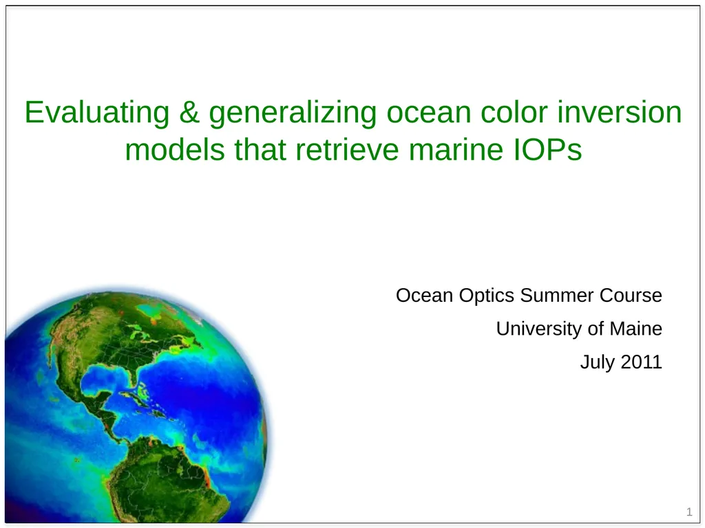
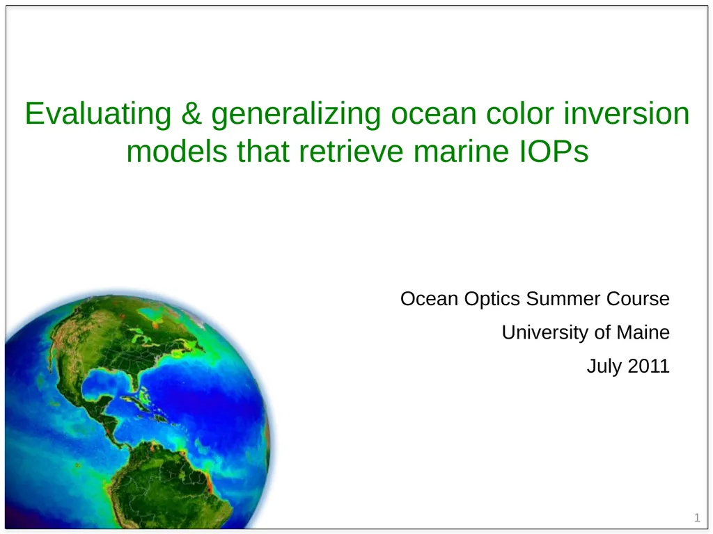
1 Evaluating & generalizing ocean color inversion models that retrieve marine IOPs Ocean Optics Summer Course
University of Maine
July 2011<br>
02
2 purpose you’re a discriminating customer …
how do you choose which algorithm (or parameterization) to use?
more importantly, how do you validate this choice?<br>
03
3 outline recent evaluation activities
review construction (& deconstruction) of a semi-analytical IOP algorithm
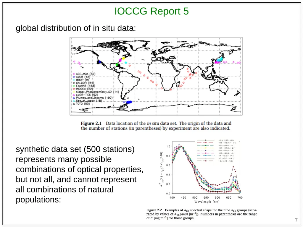
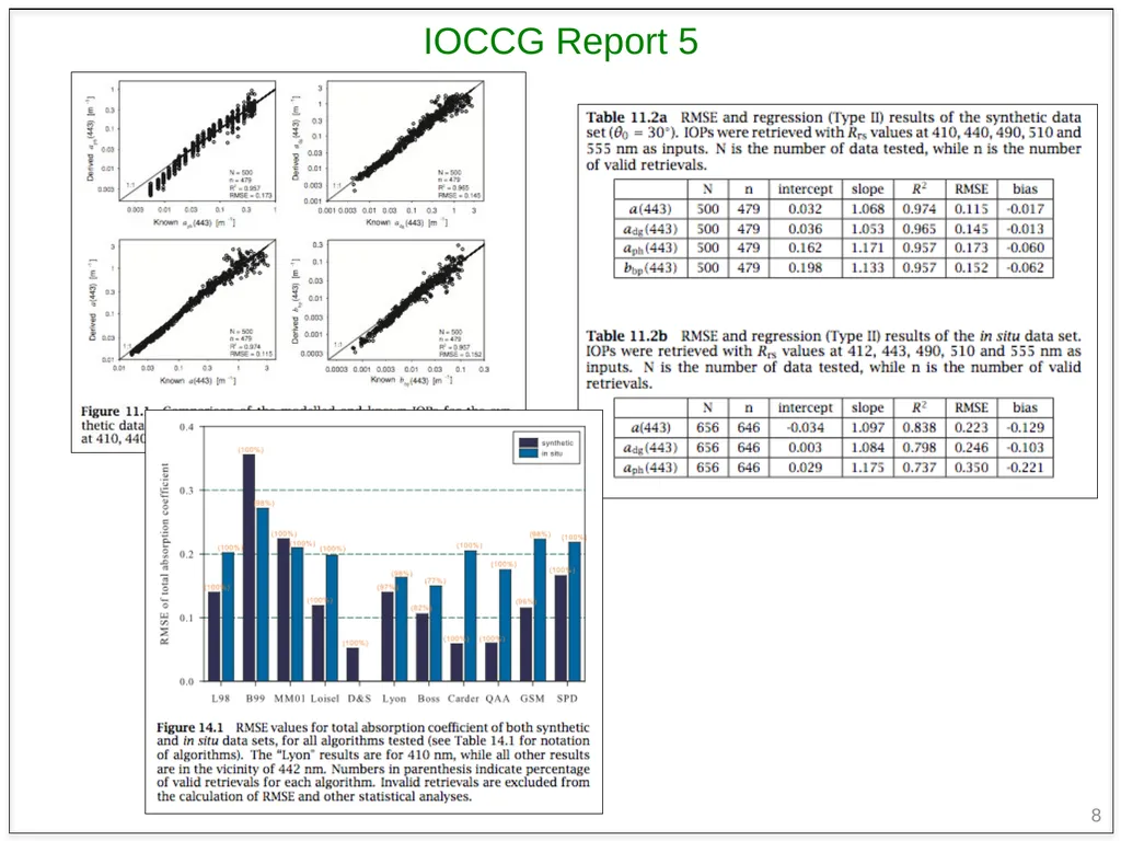
7 IOCCG Report 5 global distribution of in situ data:
synthetic data set (500 stations)
represents many possible
combinations of optical properties,
but not all, and cannot represent
all combinations of natural
populations:<br>
08
8 IOCCG Report 5<br>
09
9 purpose you’re a discriminating customer …
how do you choose which algorithm (or parameterization) to use?
more importantly, how do you validate this choice?<br>
but, most of these algorithms are very similar in their design & operation
an alternative approach to evaluating inversion algorithms might be at the level of the eigenvector (spectral shape) & statistical inversion method<br>
11
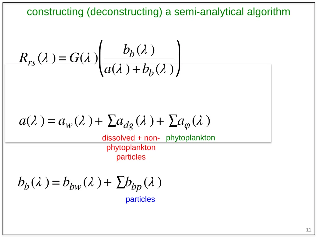
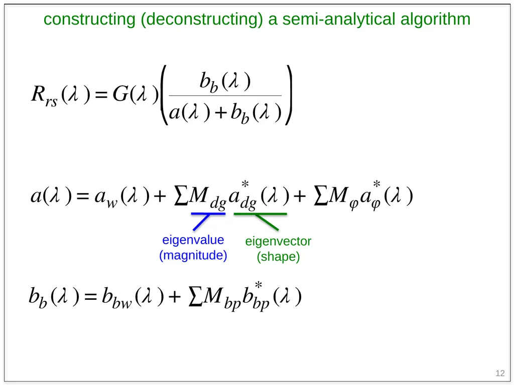
11 constructing (deconstructing) a semi-analytical algorithm<br>
12
12 constructing (deconstructing) a semi-analytical algorithm eigenvector (shape) eigenvalue (magnitude)<br>
13
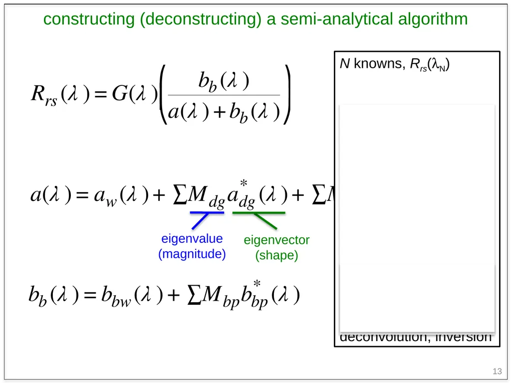
13 constructing (deconstructing) a semi-analytical algorithm eigenvector (shape) eigenvalue (magnitude) N knowns, Rrs(lN)
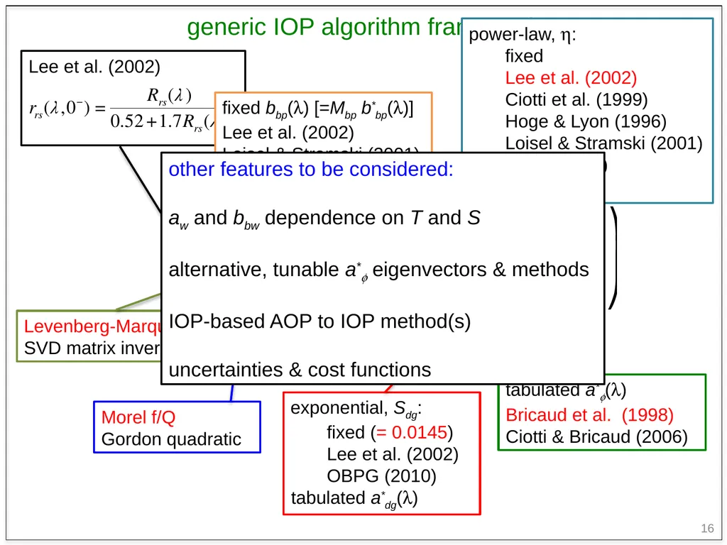
16 generic IOP algorithm framework other features to be considered:
aw and bbw dependence on T and S
alternative, tunable a*f eigenvectors & methods
IOP-based AOP to IOP method(s)
uncertainties & cost functions<br>
17
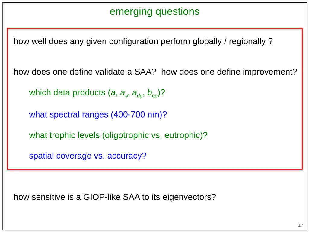
17 emerging questions how well does any given configuration perform globally / regionally ? how does one define validate a SAA? how does one define improvement?
which data products (a, af, adg, bbp)?
what spectral ranges (400-700 nm)?
what trophic levels (oligotrophic vs. eutrophic)?
spatial coverage vs. accuracy?
how sensitive is a GIOP-like SAA to its eigenvectors?<br>
18
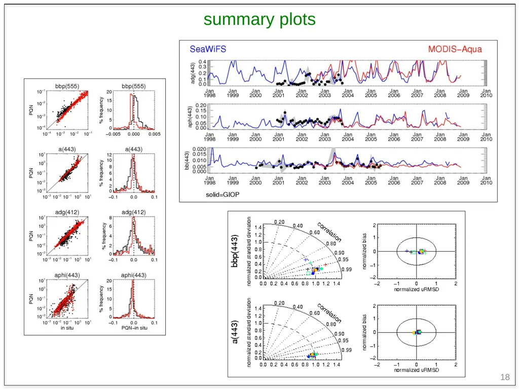
18 summary plots<br>
19
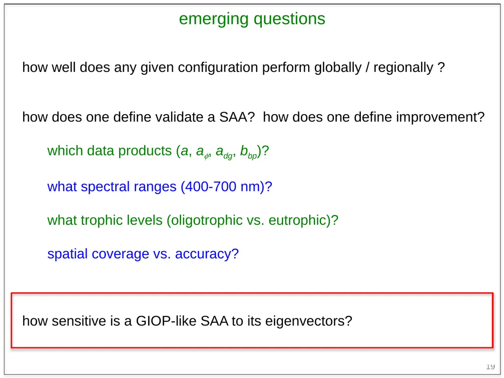
19 emerging questions how well does any given configuration perform globally / regionally ? how does one define validate a SAA? how does one define improvement?
which data products (a, af, adg, bbp)?
what spectral ranges (400-700 nm)?
what trophic levels (oligotrophic vs. eutrophic)?
spatial coverage vs. accuracy?
how sensitive is a GIOP-like SAA to its eigenvectors?<br>
20
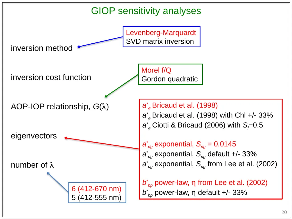
20 inversion method
inversion cost function
AOP-IOP relationship, G(l)
eigenvectors
number of l GIOP sensitivity analyses<br>
21
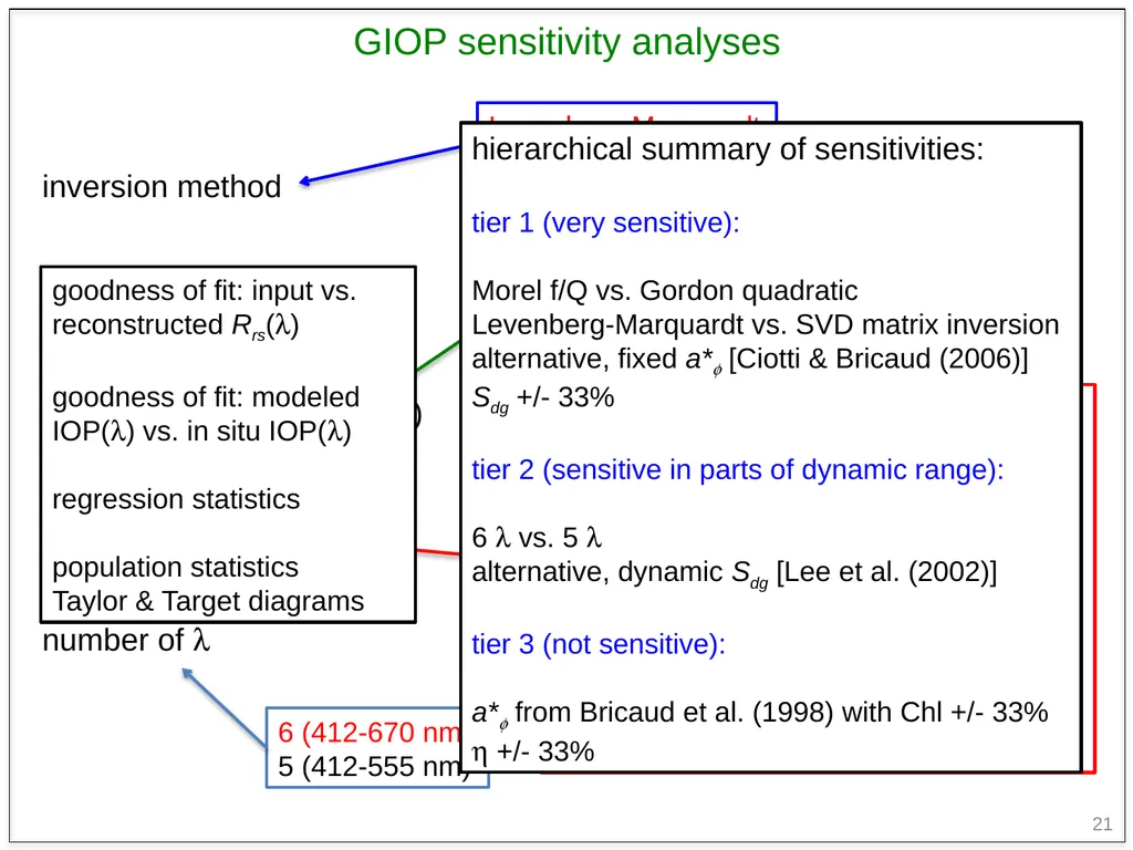
21 inversion method
inversion cost function
AOP-IOP relationship, G(l)
eigenvectors
number of l GIOP sensitivity analyses hierarchical summary of sensitivities:
tier 1 (very sensitive):
Morel f/Q vs. Gordon quadratic
Levenberg-Marquardt vs. SVD matrix inversion
alternative, fixed a*f [Ciotti & Bricaud (2006)]
Sdg +/- 33%
tier 2 (sensitive in parts of dynamic range):
6 l vs. 5 l
alternative, dynamic Sdg [Lee et al. (2002)]
tier 3 (not sensitive):
a*f from Bricaud et al. (1998) with Chl +/- 33%
h +/- 33% goodness of fit: input vs. reconstructed Rrs(l)
goodness of fit: modeled IOP(l) vs. in situ IOP(l)
regression statistics
population statistics
Taylor & Target diagrams<br>