
6.888: Lecture 4 Data Center Load Balancing



Description: 6.888: Lecture 4 Data Center Load Balancing Mohammad Alizadeh Spring 2016 1 Motivation 2 DC networks need large bisection bandwidth for distributed apps (big data, HPC, web services, etc) Leaf 1000s of server ports Multi-rooted tree
Related Topics
Download Presentation
"6.888: Lecture 4 Data Center Load Balancing" is the property of its rightful owner. Permission is granted to download and print the materials on this website for personal, non-commercial use only, and to display it on your personal computer provided you do not modify the materials and that you retain all copyright notices contained in the materials. By downloading content from our website, you accept the terms of this agreement.
Presentation Transcript
slide1. 6.888:
Lecture 4
Data Center Load Balancing Mohammad Alizadeh
Spring 2016 1<br>
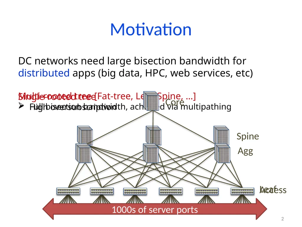
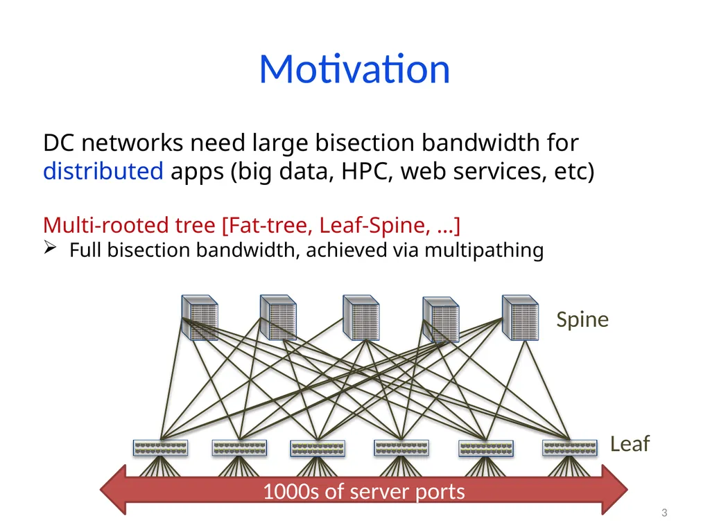
slide2. Motivation 2 DC networks need large bisection bandwidth for distributed apps (big data, HPC, web services, etc)<br>
slide3. Leaf 1000s of server ports Multi-rooted tree [Fat-tree, Leaf-Spine, …]
Full bisection bandwidth, achieved via multipathing Spine Motivation 3 DC networks need large bisection bandwidth for distributed apps (big data, HPC, web services, etc)<br>
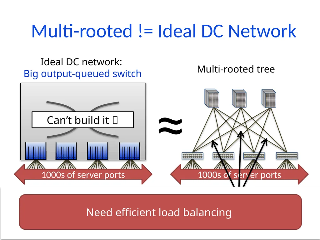
slide4. Multi-rooted != Ideal DC Network 4 No internal bottlenecks predictable
Simplifies BW management [Bw guarantees, QoS, …] Can’t build it ≈<br>
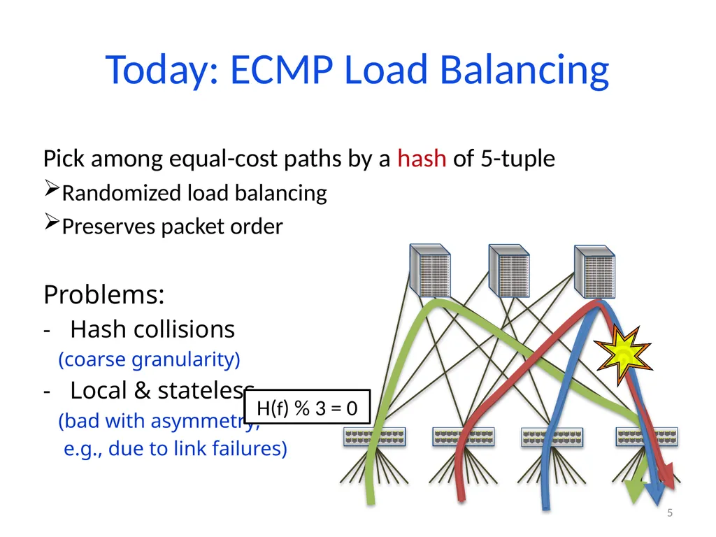
slide5. Today: ECMP Load Balancing Pick among equal-cost paths by a hash of 5-tuple
Randomized load balancing
Preserves packet order 5 Problems:
Hash collisions
(coarse granularity)
Local & stateless
(bad with asymmetry;
e.g., due to link failures) H(f) % 3 = 0<br>
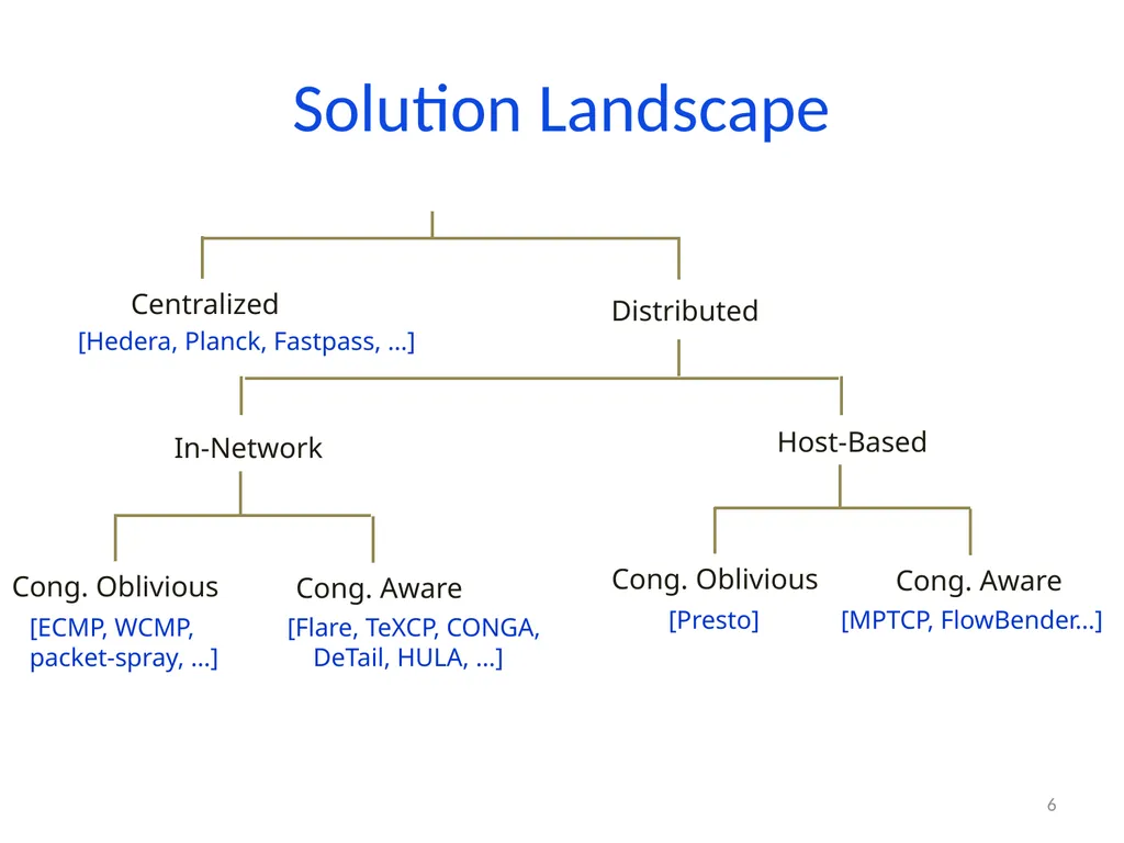
slide6. Solution Landscape 6<br>
slide7. MPTCP 7 Slides by Damon Wischik (with minor modifications)<br>
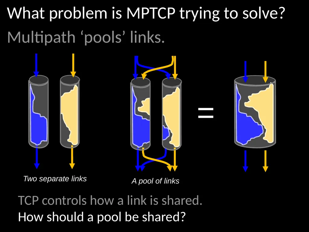
slide8. What problem is MPTCP trying to solve?
Multipath ‘pools’ links. TCP controls how a link is shared.
How should a pool be shared?<br>
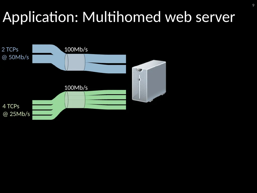
slide9. Application: Multihomed web server 9 100Mb/s 100Mb/s 2 TCPs @ 50Mb/s 4 TCPs @ 25Mb/s<br>
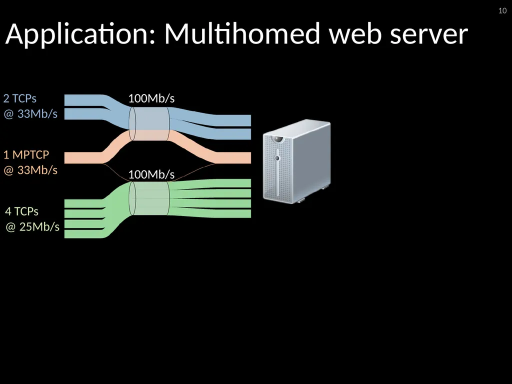
slide10. Application: Multihomed web server 10 100Mb/s 100Mb/s 2 TCPs @ 33Mb/s 1 MPTCP @ 33Mb/s 4 TCPs @ 25Mb/s<br>
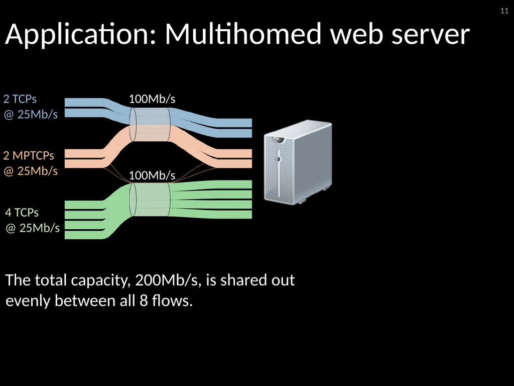
slide11. 11 100Mb/s 100Mb/s 2 TCPs @ 25Mb/s 2 MPTCPs @ 25Mb/s 4 TCPs @ 25Mb/s The total capacity, 200Mb/s, is shared out evenly between all 8 flows. Application: Multihomed web server<br>
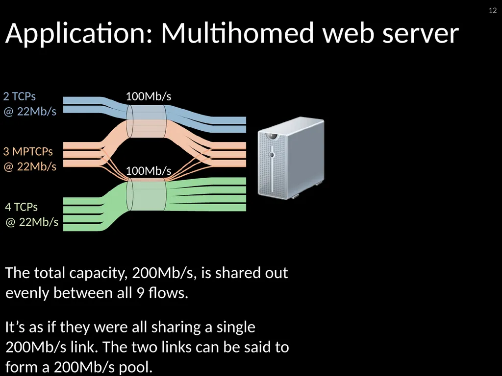
slide12. 12 100Mb/s 100Mb/s 2 TCPs @ 22Mb/s 3 MPTCPs @ 22Mb/s 4 TCPs @ 22Mb/s The total capacity, 200Mb/s, is shared out evenly between all 9 flows.
It’s as if they were all sharing a single 200Mb/s link. The two links can be said to form a 200Mb/s pool. Application: Multihomed web server<br>
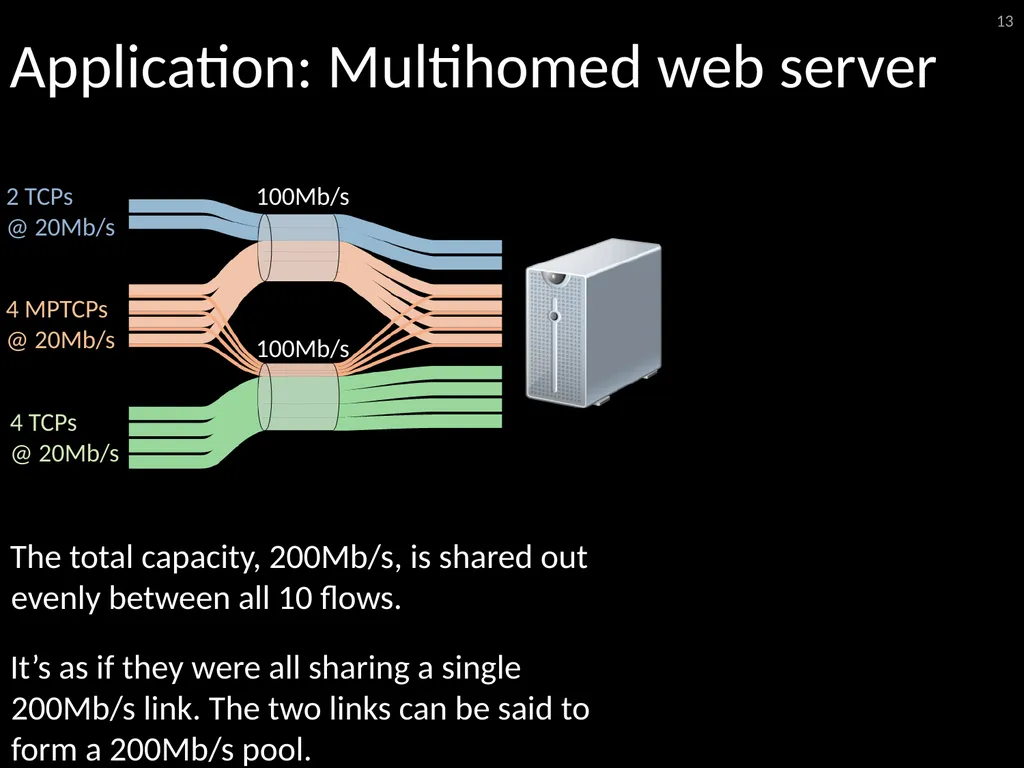
slide13. 13 100Mb/s 100Mb/s 2 TCPs @ 20Mb/s 4 MPTCPs @ 20Mb/s 4 TCPs @ 20Mb/s The total capacity, 200Mb/s, is shared out evenly between all 10 flows.
It’s as if they were all sharing a single 200Mb/s link. The two links can be said to form a 200Mb/s pool. Application: Multihomed web server<br>
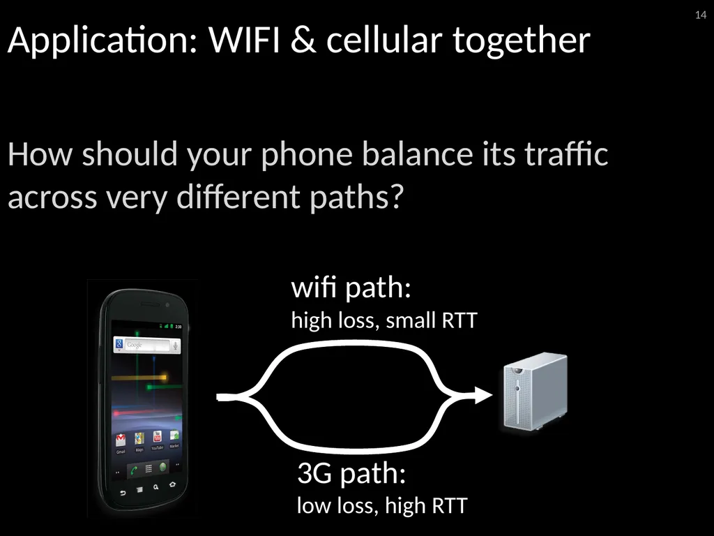
slide14. Application: WIFI & cellular together How should your phone balance its traffic across very different paths? 14 3G path: low loss, high RTT<br>
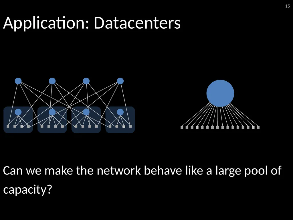
slide15. Application: Datacenters Can we make the network behave like a large pool of capacity? 15<br>
slide16. MPTCP is a general-purpose multipath replacement for TCP. 16<br>
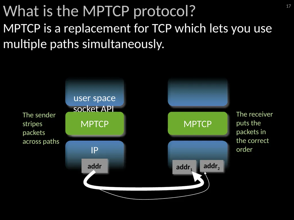
slide17. What is the MPTCP protocol? MPTCP is a replacement for TCP which lets you use multiple paths simultaneously. 17 TCP IP user space socket API MPTCP addr1 addr2 addr The sender stripes packets across paths The receiver puts the packets in the correct order<br>
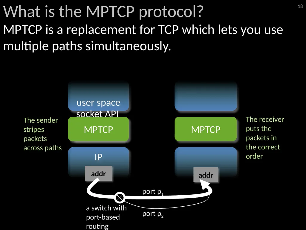
slide18. What is the MPTCP protocol? MPTCP is a replacement for TCP which lets you use multiple paths simultaneously. 18 TCP IP user space socket API MPTCP addr addr The sender stripes packets across paths The receiver puts the packets in the correct order port p1 port p2 a switch with port-based routing<br>
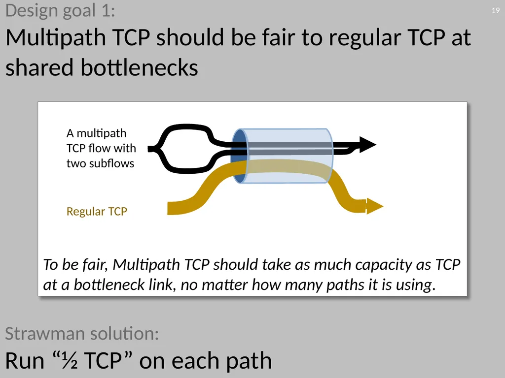
slide19. Design goal 1: Multipath TCP should be fair to regular TCP at shared bottlenecks To be fair, Multipath TCP should take as much capacity as TCP at a bottleneck link, no matter how many paths it is using. Strawman solution: Run “½ TCP” on each path A multipath TCP flow with two subflows Regular TCP 19<br>
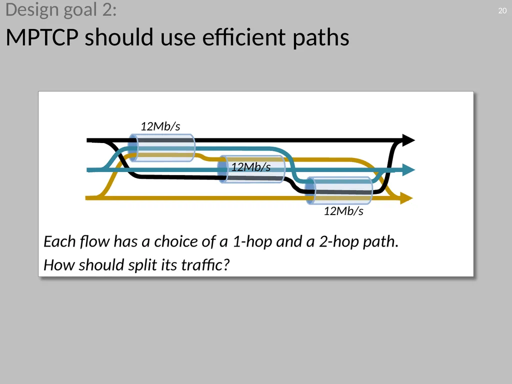
slide20. Design goal 2: MPTCP should use efficient paths Each flow has a choice of a 1-hop and a 2-hop path.
How should split its traffic? 12Mb/s 12Mb/s 12Mb/s 20<br>
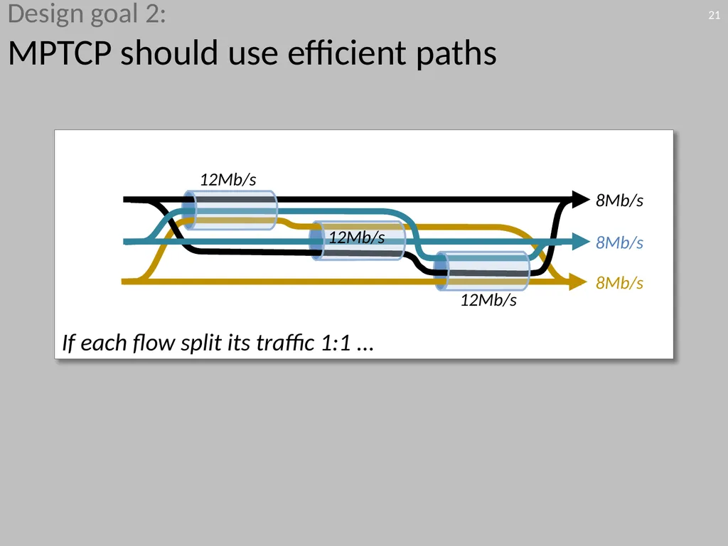
slide21. Design goal 2: MPTCP should use efficient paths If each flow split its traffic 1:1 ... 8Mb/s 8Mb/s 8Mb/s 12Mb/s 12Mb/s 12Mb/s 21<br>
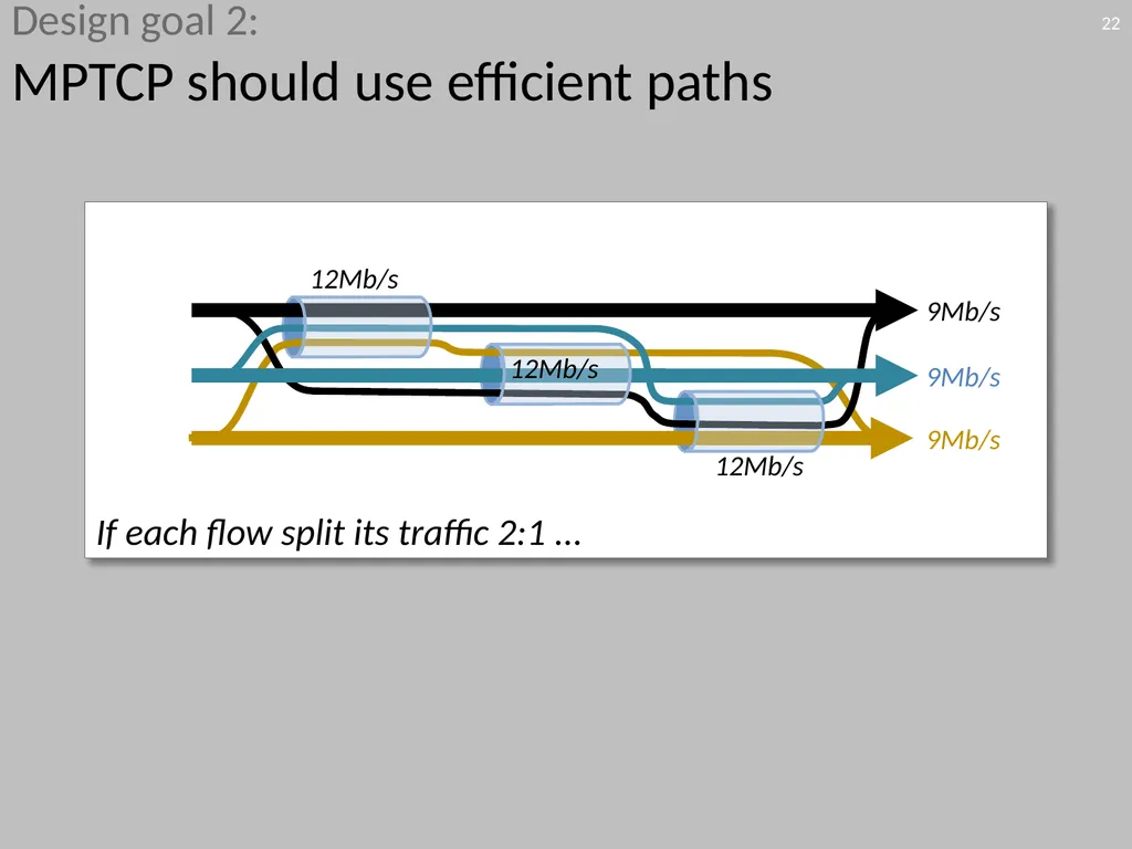
slide22. Design goal 2: MPTCP should use efficient paths If each flow split its traffic 2:1 ... 9Mb/s 9Mb/s 9Mb/s 12Mb/s 12Mb/s 12Mb/s 22<br>
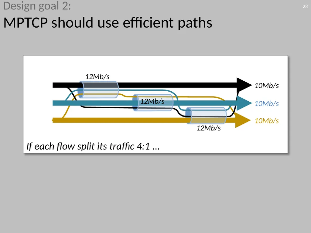
slide23. Design goal 2: MPTCP should use efficient paths If each flow split its traffic 4:1 ... 10Mb/s 10Mb/s 10Mb/s 12Mb/s 12Mb/s 12Mb/s 23<br>
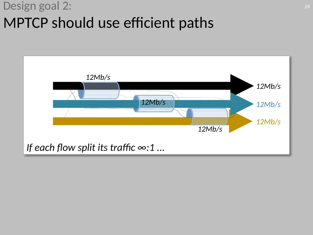
slide24. Design goal 2: MPTCP should use efficient paths If each flow split its traffic ∞:1 ... 12Mb/s 12Mb/s 12Mb/s 12Mb/s 12Mb/s 12Mb/s 24<br>
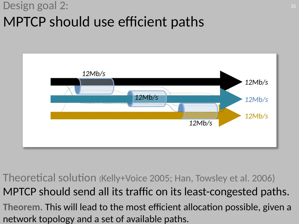
slide25. Design goal 2: MPTCP should use efficient paths 12Mb/s 12Mb/s 12Mb/s 12Mb/s 12Mb/s 12Mb/s Theoretical solution (Kelly+Voice 2005; Han, Towsley et al. 2006) MPTCP should send all its traffic on its least-congested paths. Theorem. This will lead to the most efficient allocation possible, given a network topology and a set of available paths. 25<br>
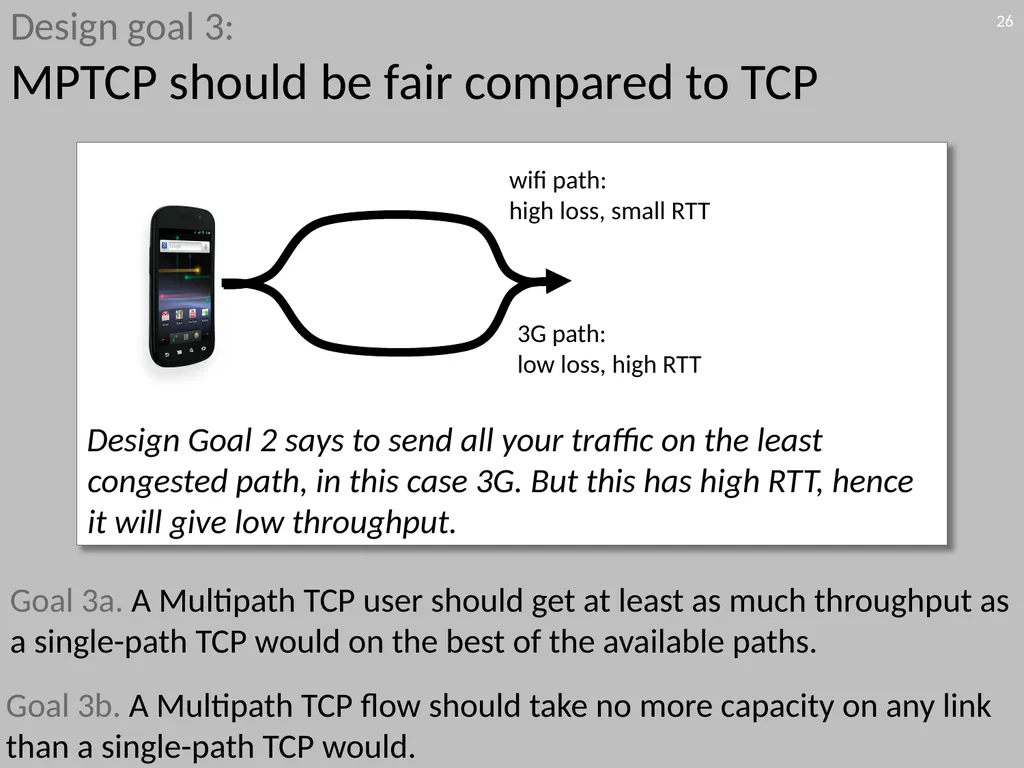
slide26. Design goal 3: MPTCP should be fair compared to TCP Design Goal 2 says to send all your traffic on the least congested path, in this case 3G. But this has high RTT, hence it will give low throughput. c d wifi path: high loss, small RTT 3G path: low loss, high RTT Goal 3a. A Multipath TCP user should get at least as much throughput as a single-path TCP would on the best of the available paths. Goal 3b. A Multipath TCP flow should take no more capacity on any link than a single-path TCP would. 26<br>
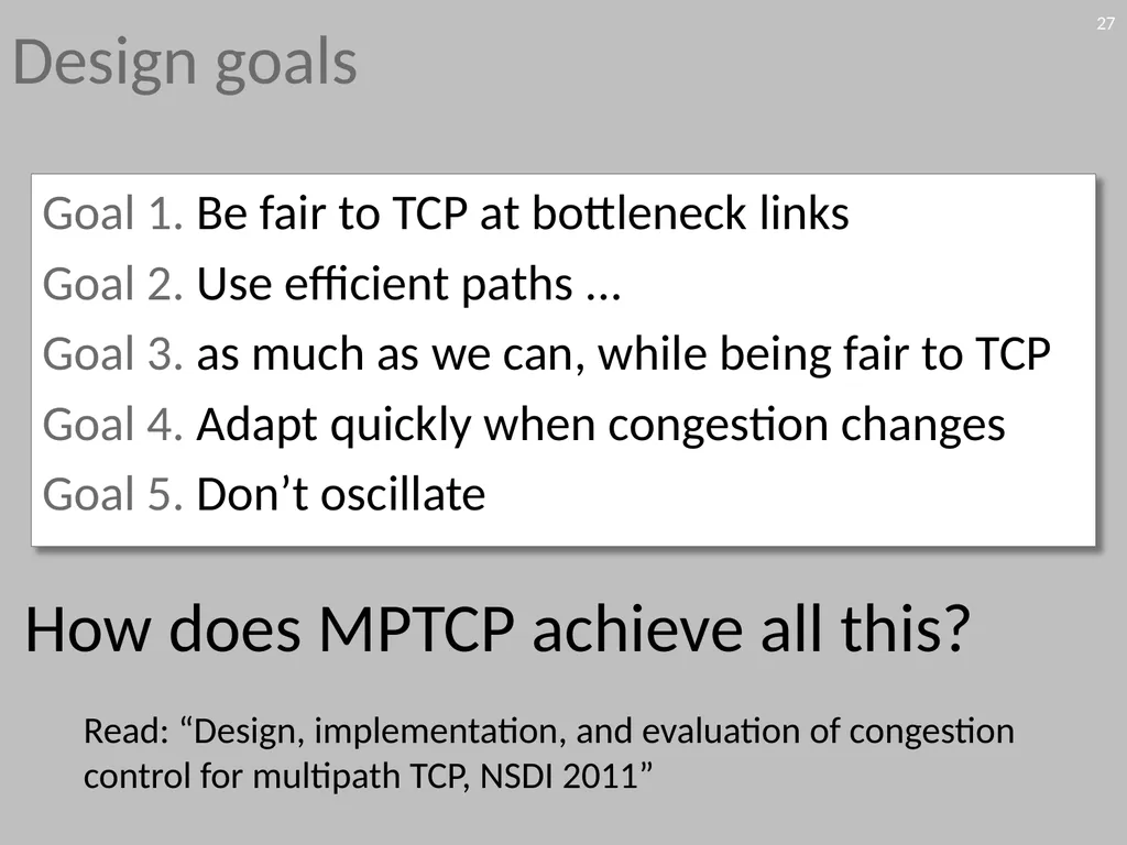
slide27. Design goals Goal 1. Be fair to TCP at bottleneck links
Goal 2. Use efficient paths ...
Goal 3. as much as we can, while being fair to TCP
Goal 4. Adapt quickly when congestion changes
Goal 5. Don’t oscillate How does MPTCP achieve all this? 27 Read: “Design, implementation, and evaluation of congestion control for multipath TCP, NSDI 2011”<br>
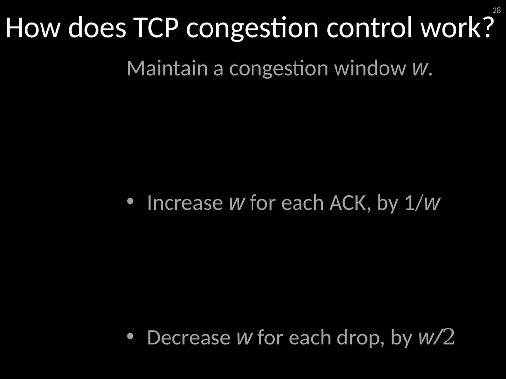
slide28. How does TCP congestion control work? Maintain a congestion window w.
Increase w for each ACK, by 1/w
Decrease w for each drop, by w/2 28<br>
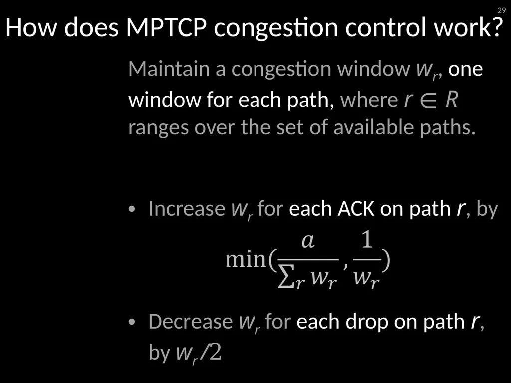
slide29. How does MPTCP congestion control work? Maintain a congestion window wr, one window for each path, where r ∊ R ranges over the set of available paths.
Increase wr for each ACK on path r, by
Decrease wr for each drop on path r, by wr /2 29<br>
slide30. Discussion 30<br>
slide31. What You Said Ravi: “An interesting point in the MPTCP paper is that they target a 'sweet spot' where there is a fair amount of traffic but the core is neither overloaded nor underloaded.” 31<br>
slide32. What You Said Hongzi: “The paper talked a bit of `probing’ to see if a link has high load and pick some other links, and there are some specific ways of assigning randomized assignment of subflows on links. I was wondering does the `power of 2 choices’ have some roles to play here?” 32<br>
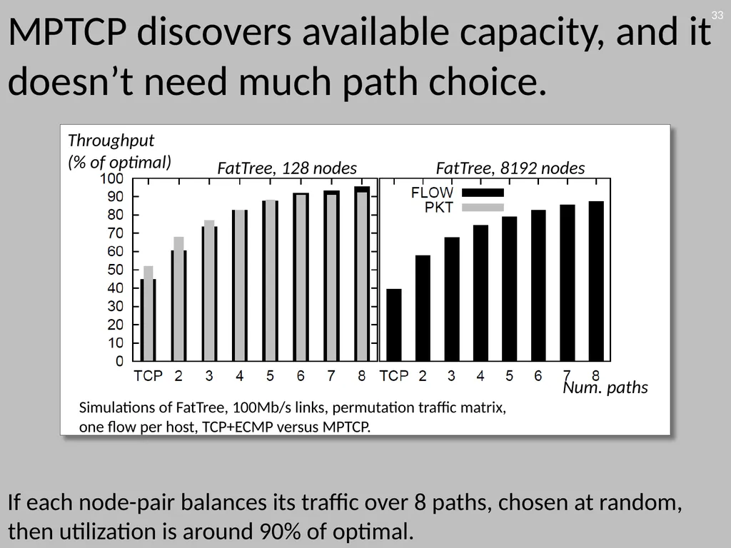
slide33. MPTCP discovers available capacity, and it doesn’t need much path choice. If each node-pair balances its traffic over 8 paths, chosen at random, then utilization is around 90% of optimal. 33 FatTree, 128 nodes FatTree, 8192 nodes Throughput (% of optimal) Num. paths Simulations of FatTree, 100Mb/s links, permutation traffic matrix, one flow per host, TCP+ECMP versus MPTCP.<br>
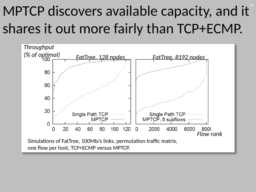
slide34. MPTCP discovers available capacity, and it shares it out more fairly than TCP+ECMP. 34 FatTree, 128 nodes FatTree, 8192 nodes Throughput (% of optimal) Flow rank Simulations of FatTree, 100Mb/s links, permutation traffic matrix, one flow per host, TCP+ECMP versus MPTCP.<br>
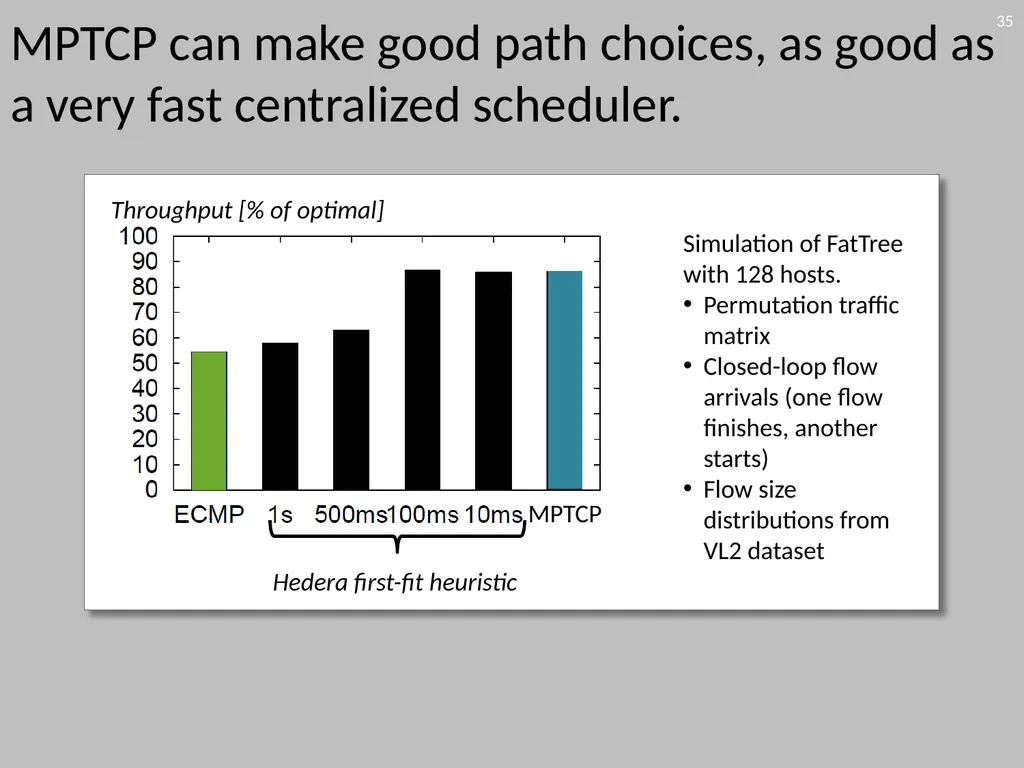
slide35. MPTCP can make good path choices, as good as a very fast centralized scheduler. 35 Simulation of FatTree with 128 hosts.
Permutation traffic matrix
Closed-loop flow arrivals (one flow finishes, another starts)
Flow size distributions from VL2 dataset Throughput [% of optimal] Hedera first-fit heuristic MPTCP<br>
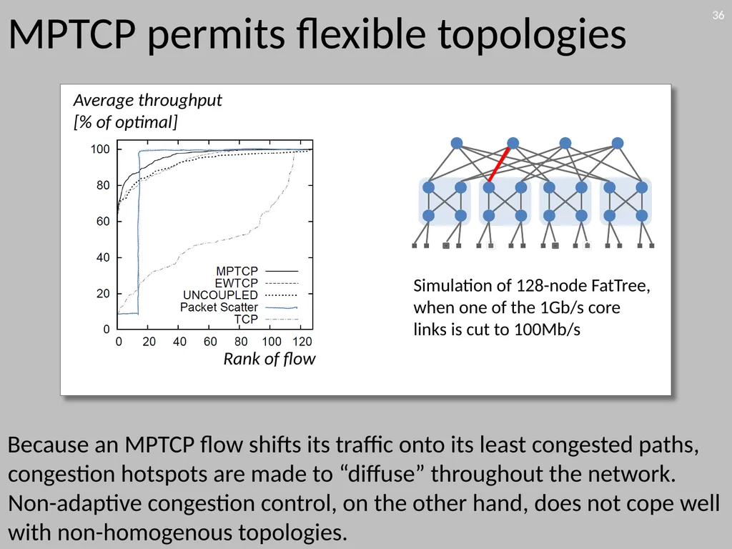
slide36. MPTCP permits flexible topologies Because an MPTCP flow shifts its traffic onto its least congested paths, congestion hotspots are made to “diffuse” throughout the network. Non-adaptive congestion control, on the other hand, does not cope well with non-homogenous topologies. 36 Average throughput [% of optimal] Rank of flow Simulation of 128-node FatTree, when one of the 1Gb/s core links is cut to 100Mb/s<br>
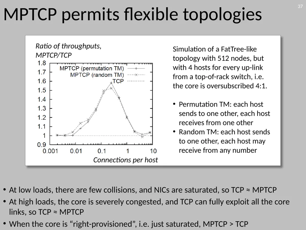
slide37. MPTCP permits flexible topologies At low loads, there are few collisions, and NICs are saturated, so TCP ≈ MPTCP
At high loads, the core is severely congested, and TCP can fully exploit all the core links, so TCP ≈ MPTCP
When the core is “right-provisioned”, i.e. just saturated, MPTCP > TCP 37 Connections per host Ratio of throughputs, MPTCP/TCP Simulation of a FatTree-like topology with 512 nodes, but with 4 hosts for every up-link from a top-of-rack switch, i.e. the core is oversubscribed 4:1.
Permutation TM: each host sends to one other, each host receives from one other
Random TM: each host sends to one other, each host may receive from any number<br>
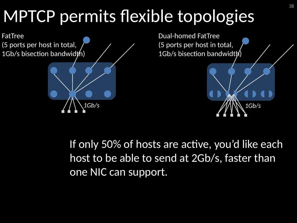
slide38. MPTCP permits flexible topologies If only 50% of hosts are active, you’d like each host to be able to send at 2Gb/s, faster than one NIC can support. 38 FatTree
(5 ports per host in total,
1Gb/s bisection bandwidth) Dual-homed FatTree
(5 ports per host in total,
1Gb/s bisection bandwidth) 1Gb/s 1Gb/s<br>
slide39. Presto 39 Adapted from slides by Keqiang He (Wisconsin)<br>
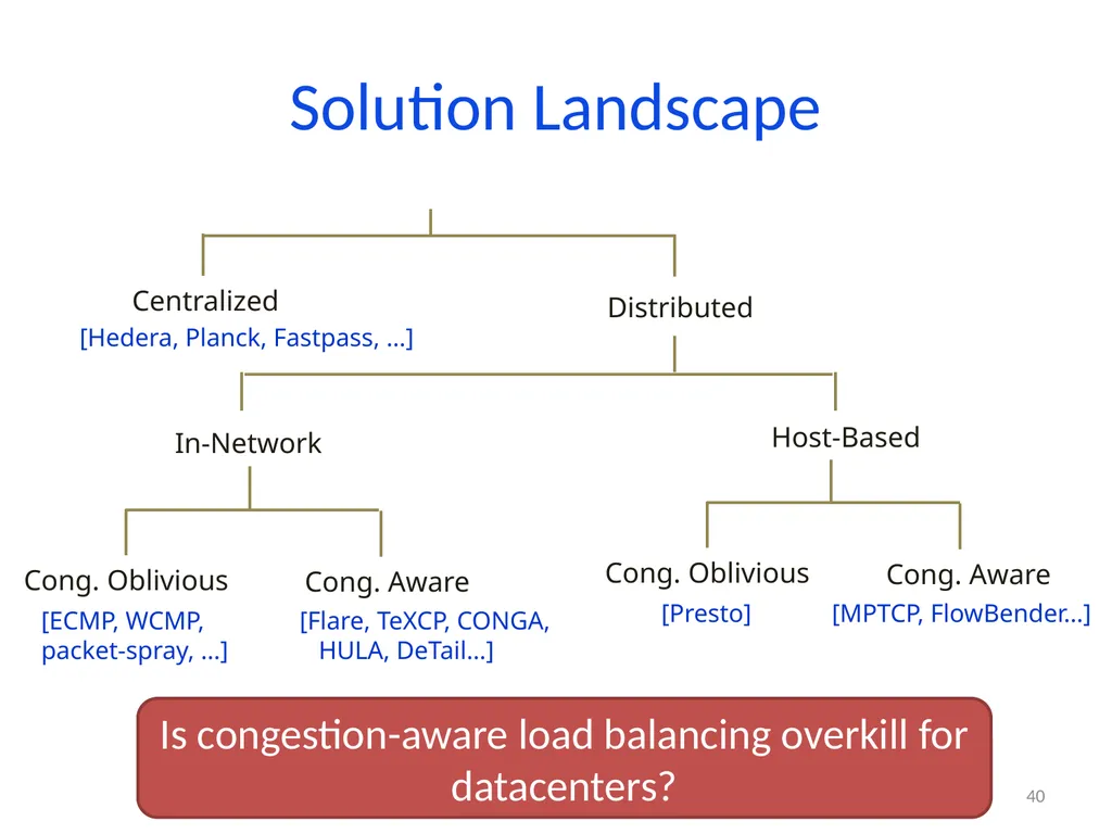
slide40. Solution Landscape 40 Is congestion-aware load balancing overkill for datacenters?<br>
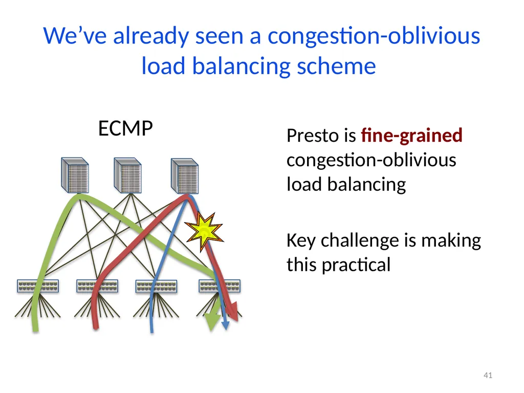
slide41. We’ve already seen a congestion-oblivious load balancing scheme 41 Presto is fine-grained congestion-oblivious
load balancing Key challenge is making this practical<br>
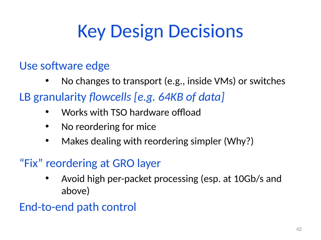
slide42. Key Design Decisions Use software edge
No changes to transport (e.g., inside VMs) or switches
LB granularity flowcells [e.g. 64KB of data]
Works with TSO hardware offload
No reordering for mice
Makes dealing with reordering simpler (Why?)
“Fix” reordering at GRO layer
Avoid high per-packet processing (esp. at 10Gb/s and above)
End-to-end path control 42<br>
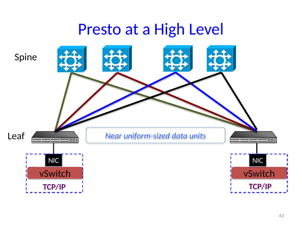
slide43. Presto at a High Level 43 vSwitch NIC NIC vSwitch TCP/IP Spine Leaf TCP/IP Near uniform-sized data units<br>
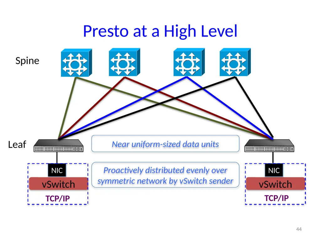
slide44. Presto at a High Level 44 vSwitch NIC NIC vSwitch TCP/IP Spine Leaf TCP/IP Proactively distributed evenly over symmetric network by vSwitch sender Near uniform-sized data units<br>
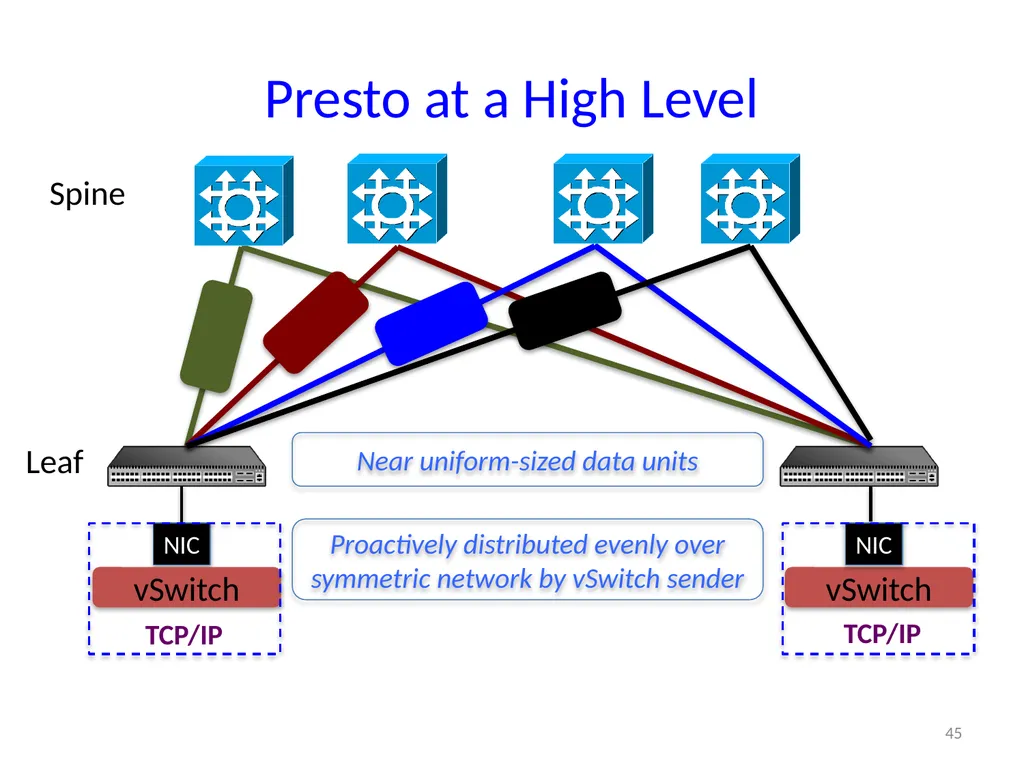
slide45. Presto at a High Level 45 vSwitch NIC NIC vSwitch TCP/IP Spine Leaf TCP/IP Proactively distributed evenly over symmetric network by vSwitch sender Near uniform-sized data units<br>
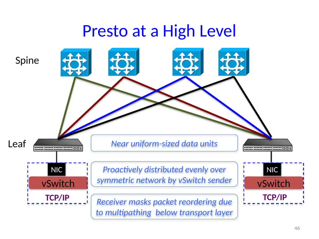
slide46. Presto at a High Level 46 vSwitch NIC NIC vSwitch TCP/IP Spine Leaf TCP/IP Receiver masks packet reordering due to multipathing below transport layer Proactively distributed evenly over symmetric network by vSwitch sender Near uniform-sized data units<br>
slide47. Discussion 47<br>
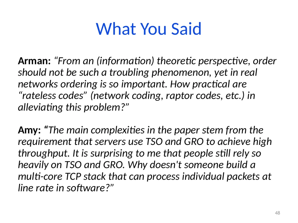
slide48. What You Said Arman: “From an (information) theoretic perspective, order should not be such a troubling phenomenon, yet in real networks ordering is so important. How practical are “rateless codes” (network coding, raptor codes, etc.) in alleviating this problem?”
Amy: “The main complexities in the paper stem from the requirement that servers use TSO and GRO to achieve high throughput. It is surprising to me that people still rely so heavily on TSO and GRO. Why doesn't someone build a multi-core TCP stack that can process individual packets at line rate in software?” 48<br>
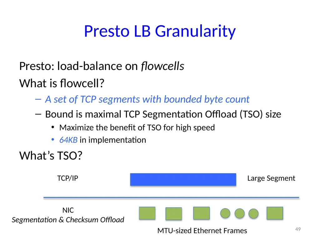
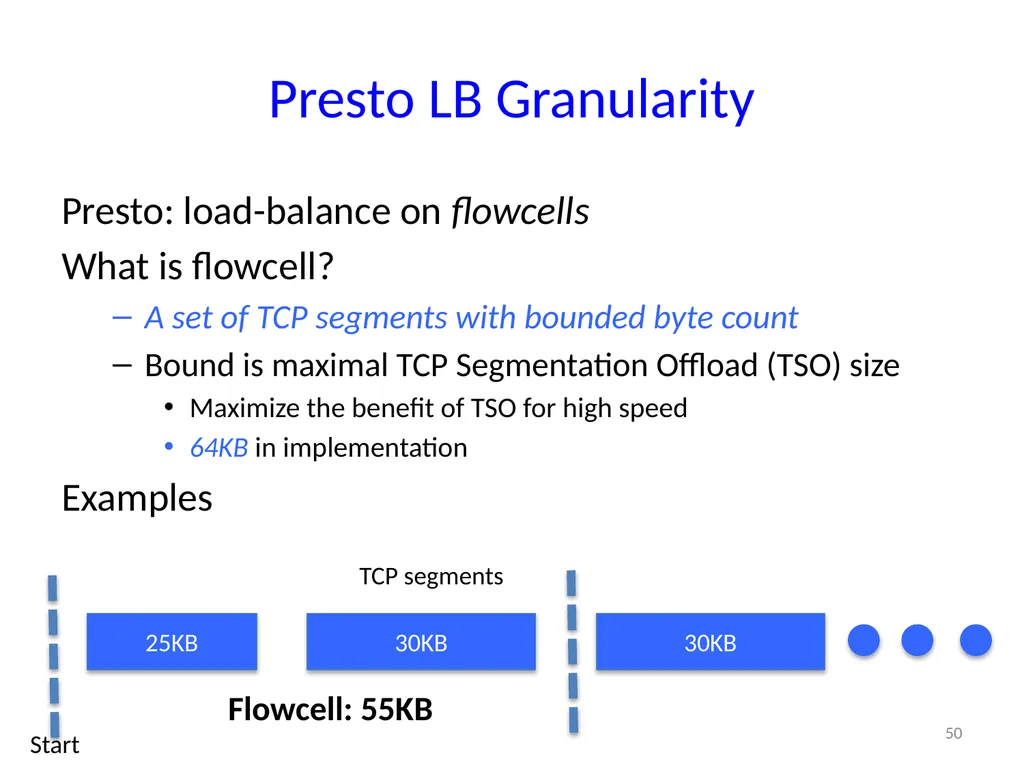
slide49. Presto LB Granularity Presto: load-balance on flowcells
What is flowcell?
A set of TCP segments with bounded byte count
Bound is maximal TCP Segmentation Offload (TSO) size
Maximize the benefit of TSO for high speed
64KB in implementation
What’s TSO? 49 TCP/IP NIC
Segmentation & Checksum Offload MTU-sized Ethernet Frames Large Segment<br>
slide50. Presto LB Granularity Presto: load-balance on flowcells
What is flowcell?
A set of TCP segments with bounded byte count
Bound is maximal TCP Segmentation Offload (TSO) size
Maximize the benefit of TSO for high speed
64KB in implementation
Examples 50 25KB 30KB 30KB Flowcell: 55KB TCP segments Start<br>
slide51. Intro to GRO Generic Receive Offload (GRO)
The reverse process of TSO 51<br>
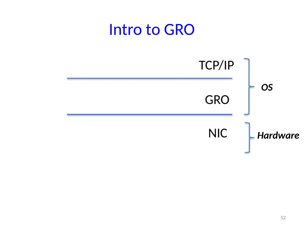
slide52. Intro to GRO TCP/IP GRO NIC 52 OS Hardware<br>
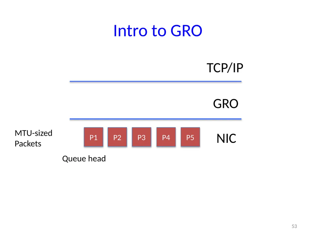
slide53. Intro to GRO TCP/IP GRO NIC MTU-sized
Packets 53 P2 P3 P4 P5 P1 Queue head<br>
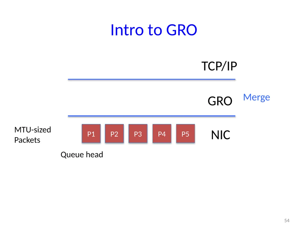
slide54. Intro to GRO TCP/IP GRO NIC MTU-sized
Packets 54 P2 P3 P4 P5 P1 Merge Queue head<br>
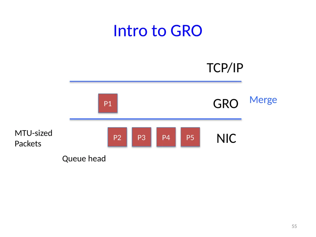
slide55. Intro to GRO TCP/IP GRO NIC MTU-sized
Packets 55 P2 P3 P4 P5 P1 Merge Queue head<br>
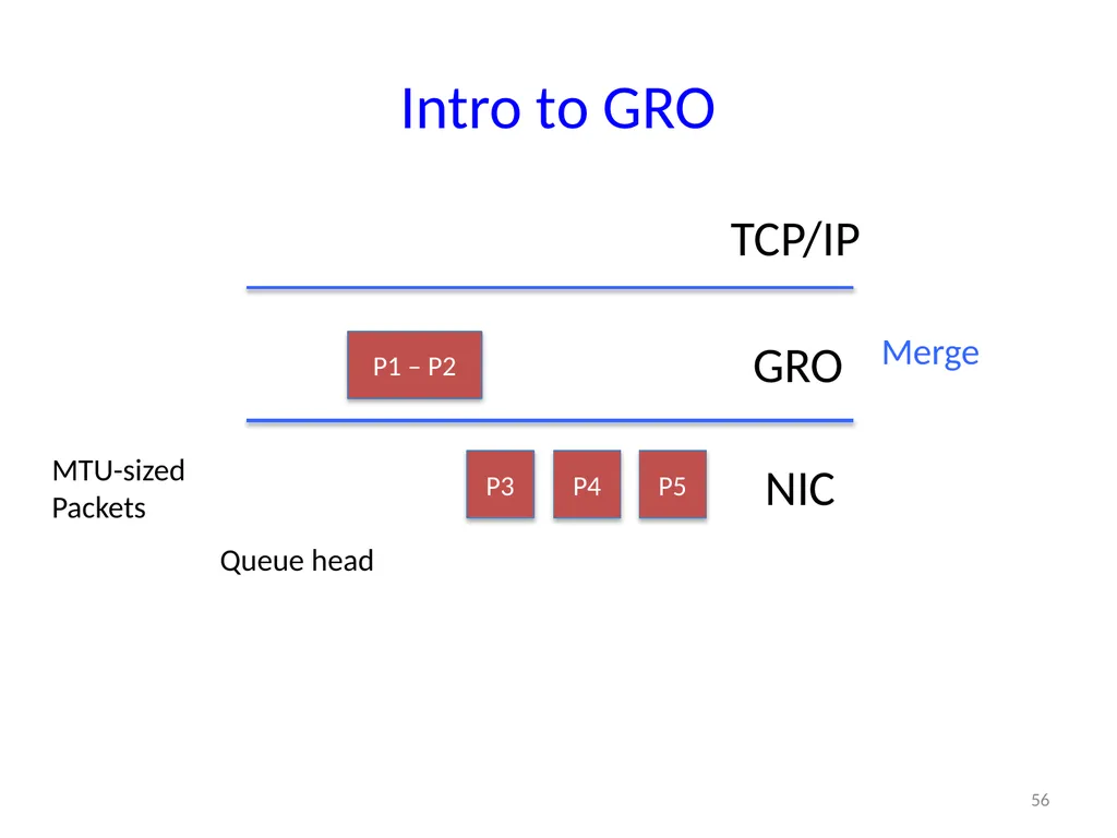
slide56. Intro to GRO TCP/IP GRO NIC MTU-sized
Packets 56 P3 P4 P5 P1 – P2 Merge Queue head<br>
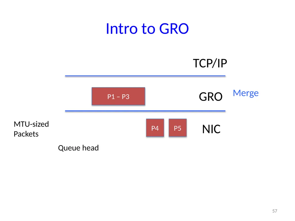
slide57. Intro to GRO TCP/IP GRO NIC MTU-sized
Packets 57 P4 P5 P1 – P3 Merge Queue head<br>
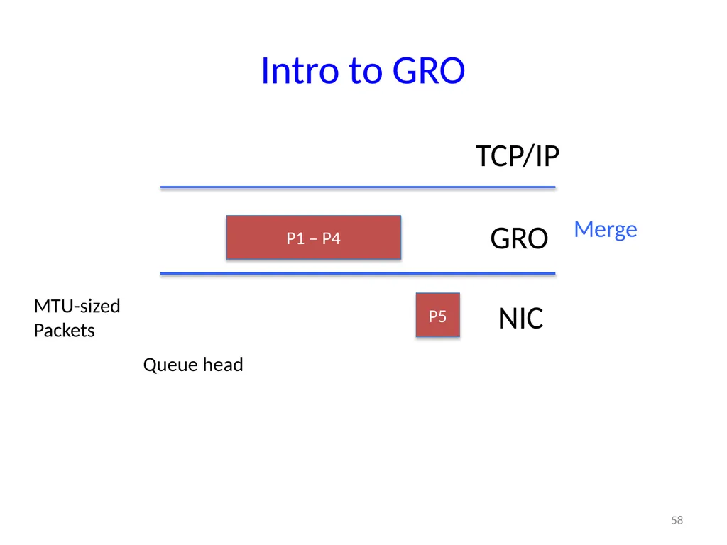
slide58. Intro to GRO TCP/IP GRO NIC MTU-sized
Packets 58 P5 P1 – P4 Merge Queue head<br>
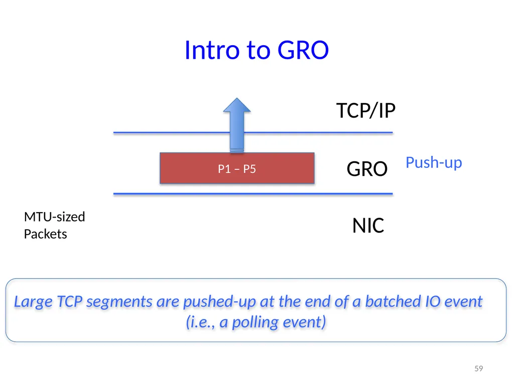
slide59. Intro to GRO TCP/IP GRO NIC MTU-sized
Packets 59 P1 – P5 Push-up Large TCP segments are pushed-up at the end of a batched IO event
(i.e., a polling event)<br>
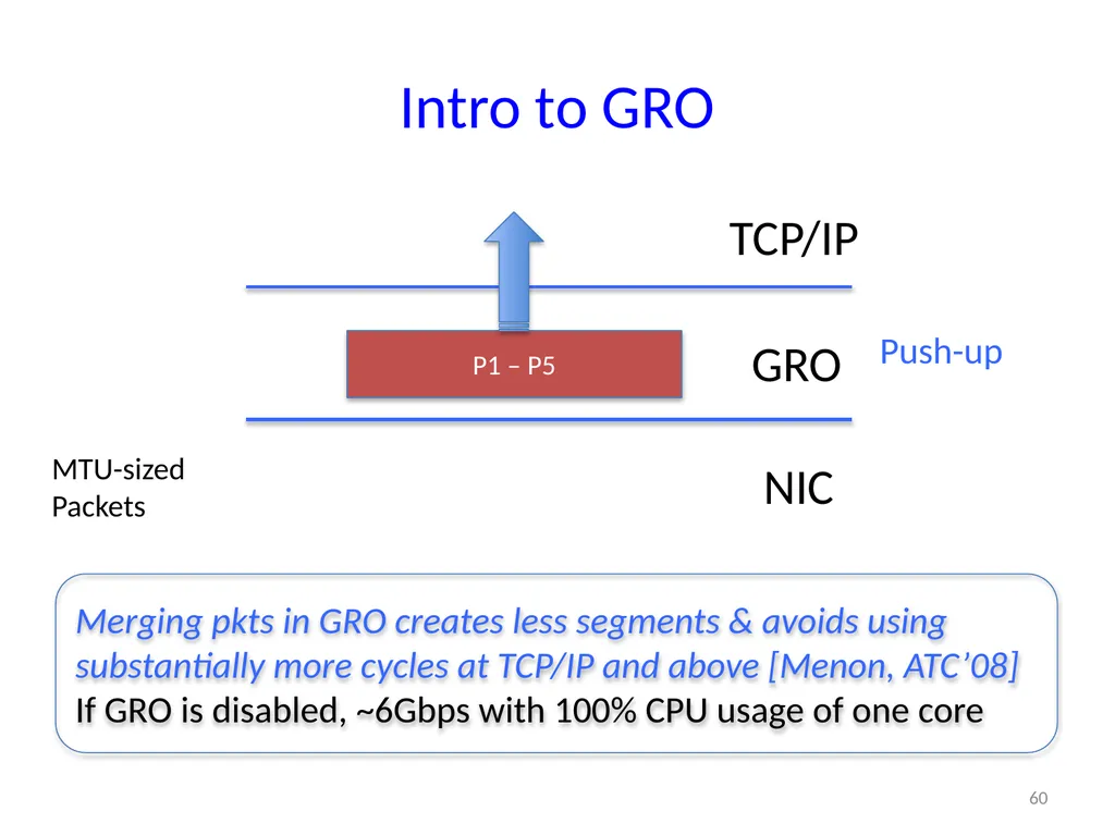
slide60. Intro to GRO TCP/IP GRO NIC MTU-sized
Packets 60 P1 – P5 Push-up Merging pkts in GRO creates less segments & avoids using substantially more cycles at TCP/IP and above [Menon, ATC’08]
If GRO is disabled, ~6Gbps with 100% CPU usage of one core<br>
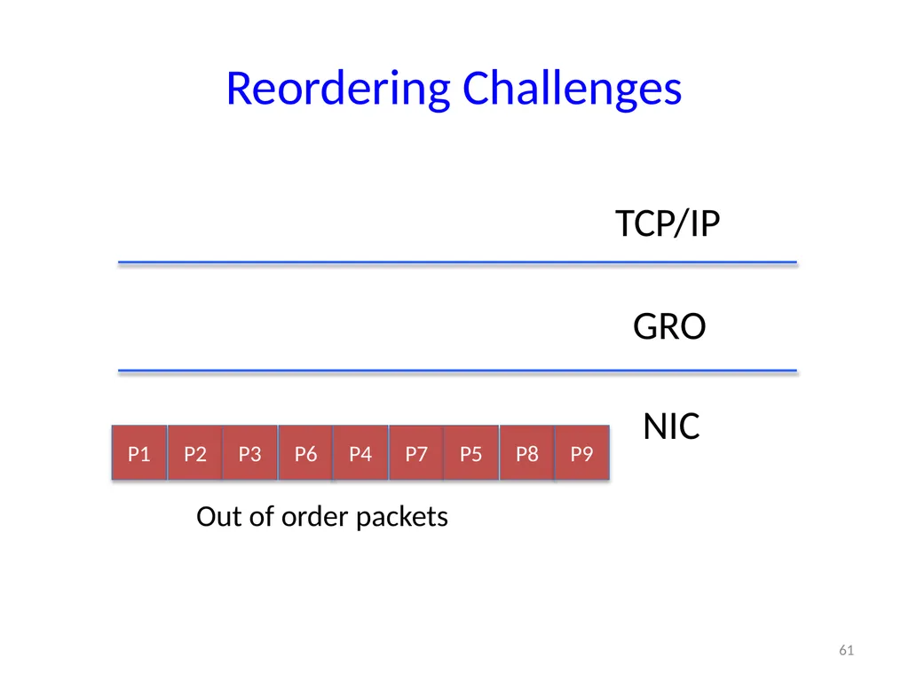
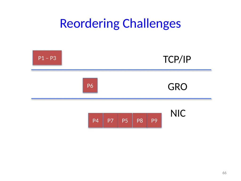
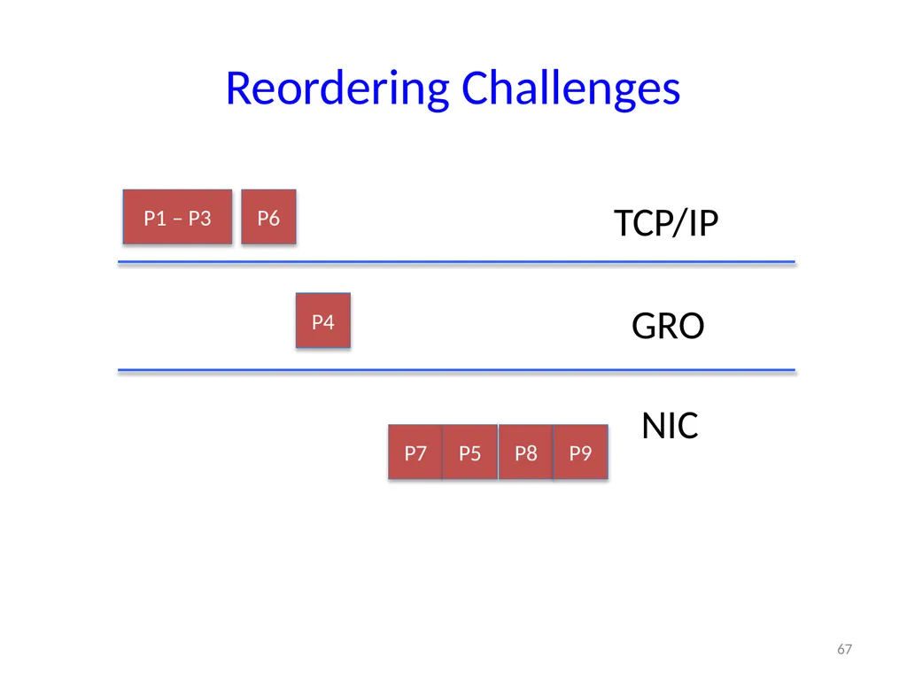
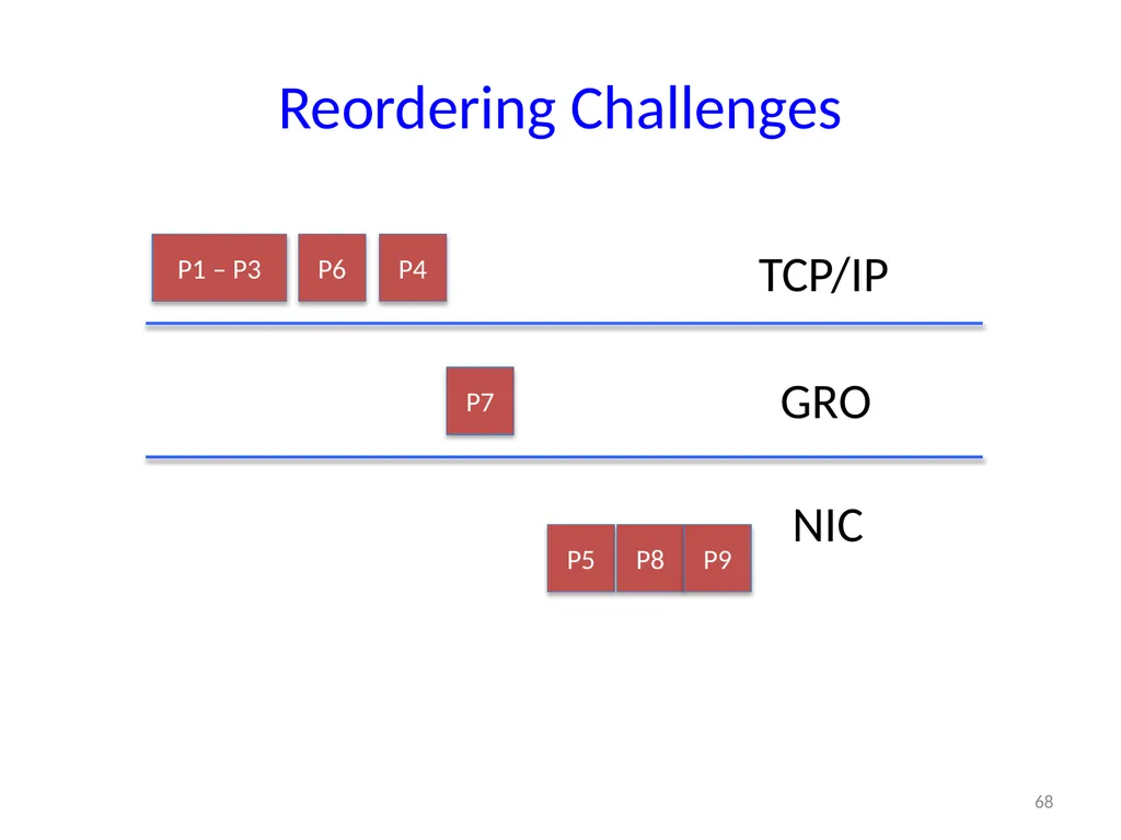
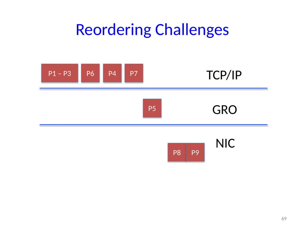
slide61. Reordering Challenges 61 P1 P2 P3 P6 P4 P7 P5 P8 P9 TCP/IP GRO NIC Out of order packets<br>
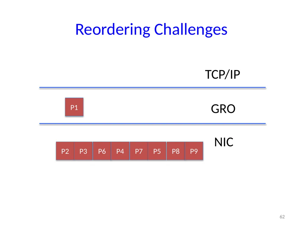
slide62. Reordering Challenges 62 P1 P2 P3 P6 P4 P7 P5 P8 P9 TCP/IP GRO NIC<br>
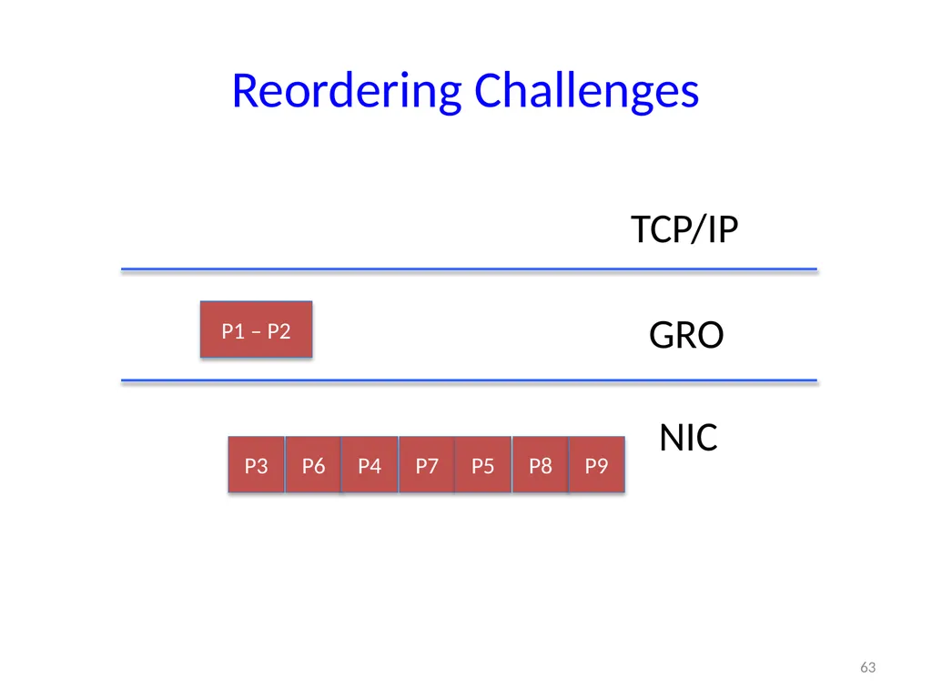
slide63. Reordering Challenges 63 P1 – P2 P3 P6 P4 P7 P5 P8 P9 TCP/IP GRO NIC<br>
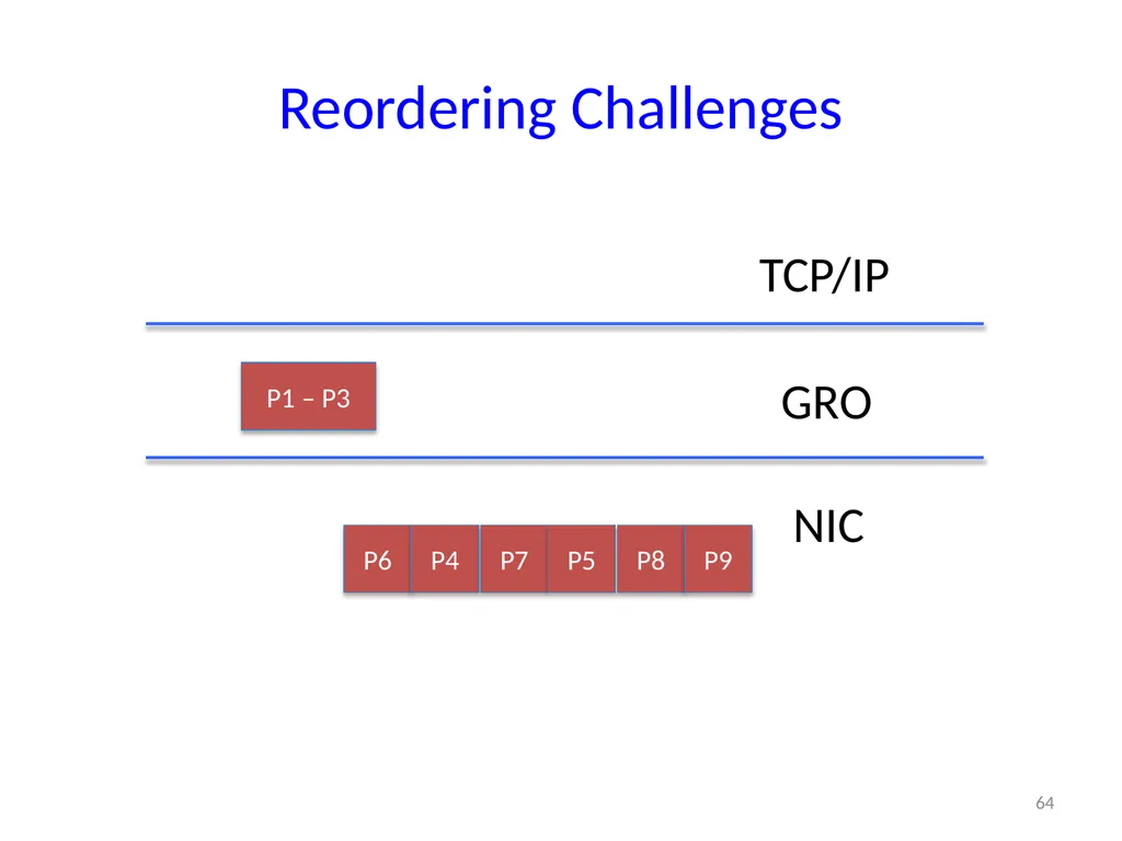
slide64. Reordering Challenges 64 P1 – P3 P6 P4 P7 P5 P8 P9 TCP/IP GRO NIC<br>
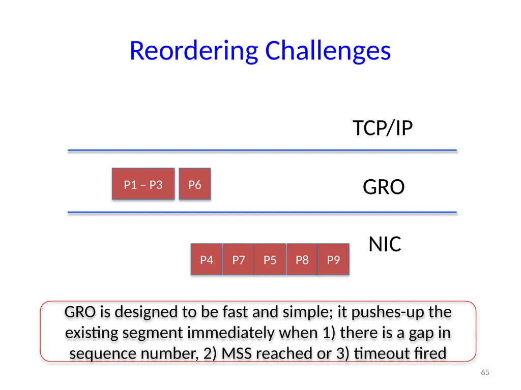
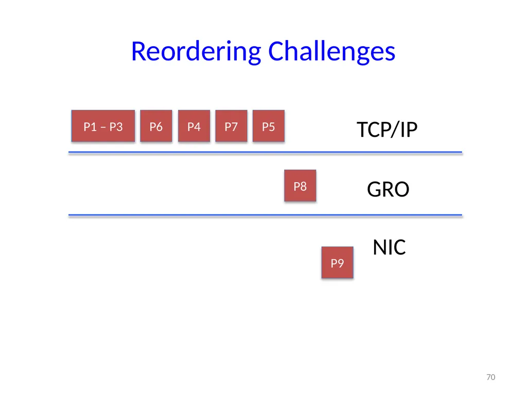
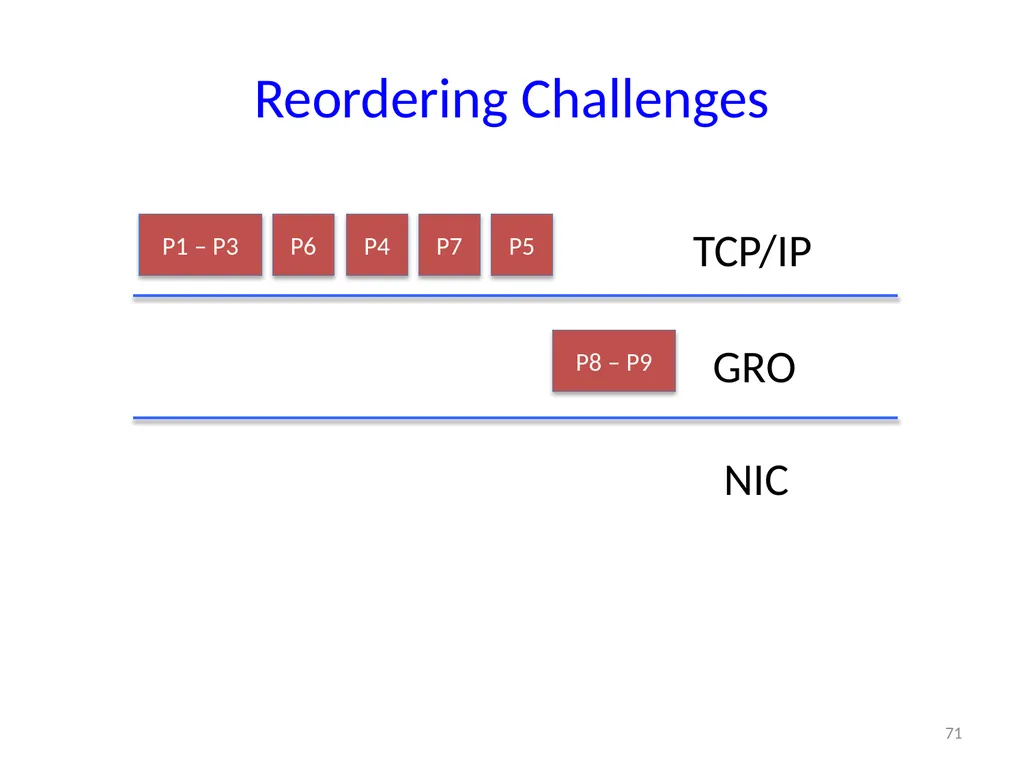
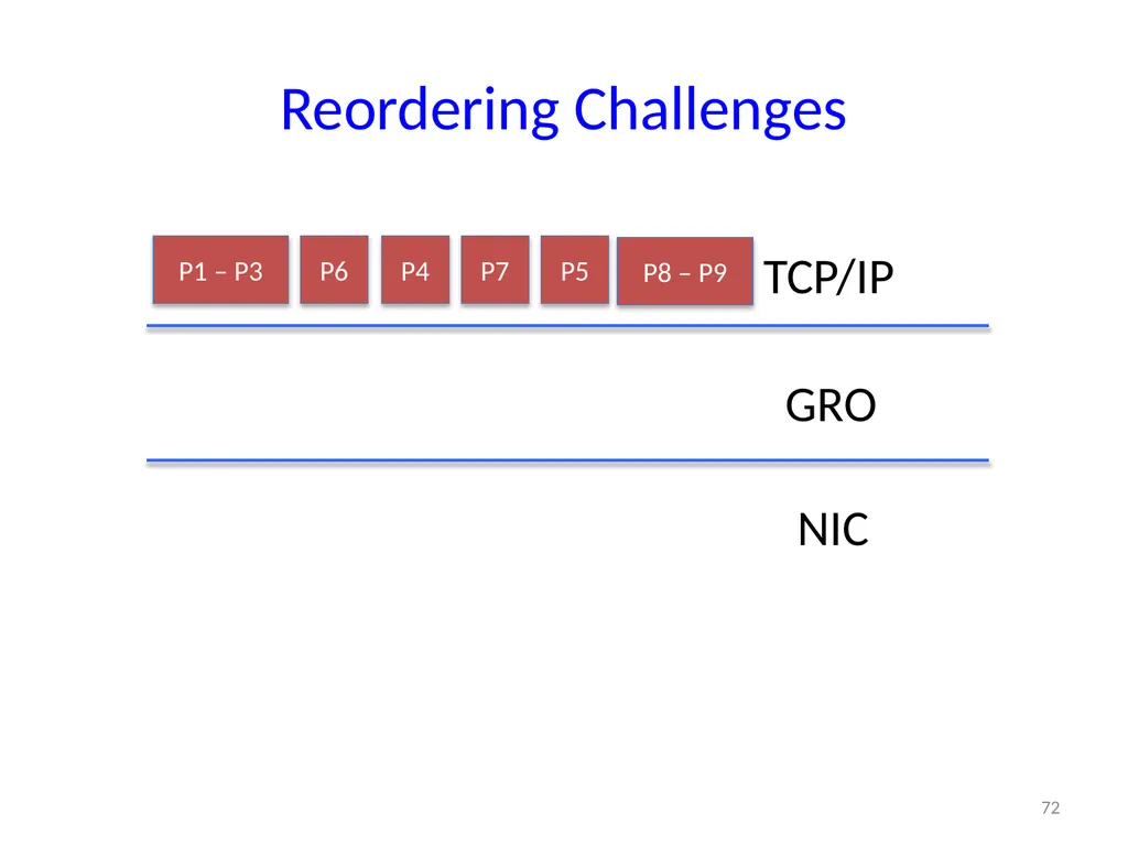
slide65. Reordering Challenges 65 P1 – P3 P6 P4 P7 P5 P8 P9 TCP/IP GRO NIC GRO is designed to be fast and simple; it pushes-up the existing segment immediately when 1) there is a gap in sequence number, 2) MSS reached or 3) timeout fired<br>
slide66. Reordering Challenges 66 P1 – P3 P6 P4 P7 P5 P8 P9 TCP/IP GRO NIC<br>
slide67. Reordering Challenges 67 P1 – P3 P6 P4 P7 P5 P8 P9 TCP/IP GRO NIC<br>
slide68. Reordering Challenges 68 P1 – P3 P6 P4 P7 P5 P8 P9 TCP/IP GRO NIC<br>
slide69. Reordering Challenges 69 P1 – P3 P6 P4 P7 P5 P8 P9 TCP/IP GRO NIC<br>
slide70. Reordering Challenges 70 P1 – P3 P6 P4 P7 P5 P8 P9 TCP/IP GRO NIC<br>
slide71. Reordering Challenges 71 P1 – P3 P6 P4 P7 P5 P8 – P9 TCP/IP GRO NIC<br>
slide72. Reordering Challenges 72 P1 – P3 P6 P4 P7 P5 P8 – P9 TCP/IP GRO NIC<br>
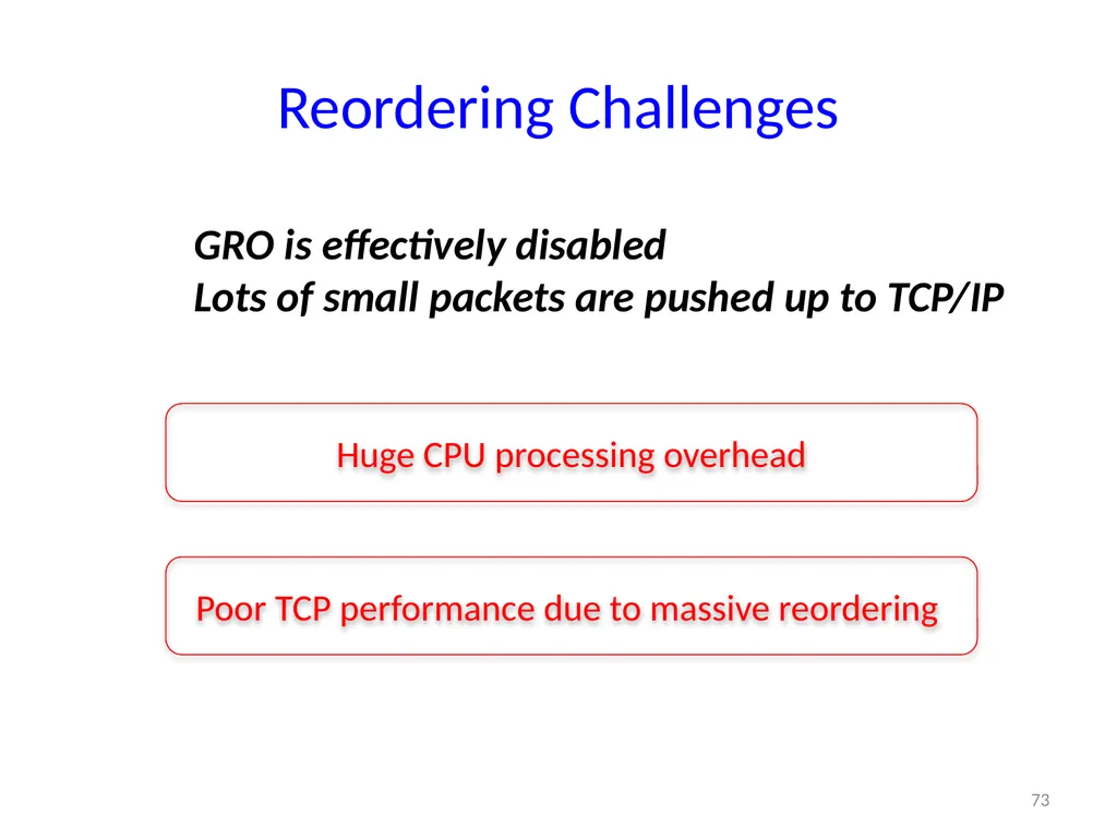
slide73. Reordering Challenges GRO is effectively disabled
Lots of small packets are pushed up to TCP/IP 73 Huge CPU processing overhead Poor TCP performance due to massive reordering<br>
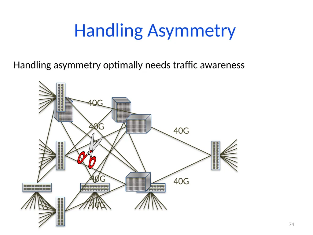
slide74. Handling Asymmetry 74 40G Handling asymmetry optimally needs traffic awareness<br>
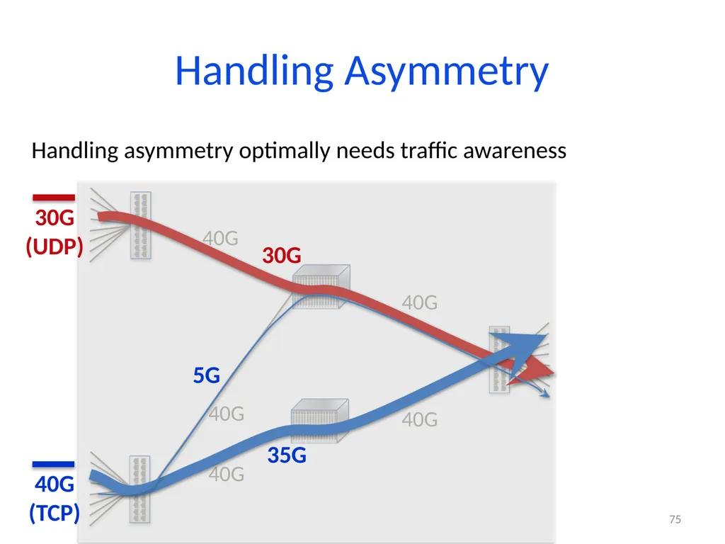
slide75. 75 30G Handling Asymmetry Handling asymmetry optimally needs traffic awareness 35G 5G<br>
slide76. 76<br>
Spring 2016 1<br>
slide2. Motivation 2 DC networks need large bisection bandwidth for distributed apps (big data, HPC, web services, etc)<br>
slide3. Leaf 1000s of server ports Multi-rooted tree [Fat-tree, Leaf-Spine, …]
Full bisection bandwidth, achieved via multipathing Spine Motivation 3 DC networks need large bisection bandwidth for distributed apps (big data, HPC, web services, etc)<br>
slide4. Multi-rooted != Ideal DC Network 4 No internal bottlenecks predictable
Simplifies BW management [Bw guarantees, QoS, …] Can’t build it ≈<br>
slide5. Today: ECMP Load Balancing Pick among equal-cost paths by a hash of 5-tuple
Randomized load balancing
Preserves packet order 5 Problems:
Hash collisions
(coarse granularity)
Local & stateless
(bad with asymmetry;
e.g., due to link failures) H(f) % 3 = 0<br>
slide6. Solution Landscape 6<br>
slide7. MPTCP 7 Slides by Damon Wischik (with minor modifications)<br>
slide8. What problem is MPTCP trying to solve?
Multipath ‘pools’ links. TCP controls how a link is shared.
How should a pool be shared?<br>
slide9. Application: Multihomed web server 9 100Mb/s 100Mb/s 2 TCPs @ 50Mb/s 4 TCPs @ 25Mb/s<br>
slide10. Application: Multihomed web server 10 100Mb/s 100Mb/s 2 TCPs @ 33Mb/s 1 MPTCP @ 33Mb/s 4 TCPs @ 25Mb/s<br>
slide11. 11 100Mb/s 100Mb/s 2 TCPs @ 25Mb/s 2 MPTCPs @ 25Mb/s 4 TCPs @ 25Mb/s The total capacity, 200Mb/s, is shared out evenly between all 8 flows. Application: Multihomed web server<br>
slide12. 12 100Mb/s 100Mb/s 2 TCPs @ 22Mb/s 3 MPTCPs @ 22Mb/s 4 TCPs @ 22Mb/s The total capacity, 200Mb/s, is shared out evenly between all 9 flows.
It’s as if they were all sharing a single 200Mb/s link. The two links can be said to form a 200Mb/s pool. Application: Multihomed web server<br>
slide13. 13 100Mb/s 100Mb/s 2 TCPs @ 20Mb/s 4 MPTCPs @ 20Mb/s 4 TCPs @ 20Mb/s The total capacity, 200Mb/s, is shared out evenly between all 10 flows.
It’s as if they were all sharing a single 200Mb/s link. The two links can be said to form a 200Mb/s pool. Application: Multihomed web server<br>
slide14. Application: WIFI & cellular together How should your phone balance its traffic across very different paths? 14 3G path: low loss, high RTT<br>
slide15. Application: Datacenters Can we make the network behave like a large pool of capacity? 15<br>
slide16. MPTCP is a general-purpose multipath replacement for TCP. 16<br>
slide17. What is the MPTCP protocol? MPTCP is a replacement for TCP which lets you use multiple paths simultaneously. 17 TCP IP user space socket API MPTCP addr1 addr2 addr The sender stripes packets across paths The receiver puts the packets in the correct order<br>
slide18. What is the MPTCP protocol? MPTCP is a replacement for TCP which lets you use multiple paths simultaneously. 18 TCP IP user space socket API MPTCP addr addr The sender stripes packets across paths The receiver puts the packets in the correct order port p1 port p2 a switch with port-based routing<br>
slide19. Design goal 1: Multipath TCP should be fair to regular TCP at shared bottlenecks To be fair, Multipath TCP should take as much capacity as TCP at a bottleneck link, no matter how many paths it is using. Strawman solution: Run “½ TCP” on each path A multipath TCP flow with two subflows Regular TCP 19<br>
slide20. Design goal 2: MPTCP should use efficient paths Each flow has a choice of a 1-hop and a 2-hop path.
How should split its traffic? 12Mb/s 12Mb/s 12Mb/s 20<br>
slide21. Design goal 2: MPTCP should use efficient paths If each flow split its traffic 1:1 ... 8Mb/s 8Mb/s 8Mb/s 12Mb/s 12Mb/s 12Mb/s 21<br>
slide22. Design goal 2: MPTCP should use efficient paths If each flow split its traffic 2:1 ... 9Mb/s 9Mb/s 9Mb/s 12Mb/s 12Mb/s 12Mb/s 22<br>
slide23. Design goal 2: MPTCP should use efficient paths If each flow split its traffic 4:1 ... 10Mb/s 10Mb/s 10Mb/s 12Mb/s 12Mb/s 12Mb/s 23<br>
slide24. Design goal 2: MPTCP should use efficient paths If each flow split its traffic ∞:1 ... 12Mb/s 12Mb/s 12Mb/s 12Mb/s 12Mb/s 12Mb/s 24<br>
slide25. Design goal 2: MPTCP should use efficient paths 12Mb/s 12Mb/s 12Mb/s 12Mb/s 12Mb/s 12Mb/s Theoretical solution (Kelly+Voice 2005; Han, Towsley et al. 2006) MPTCP should send all its traffic on its least-congested paths. Theorem. This will lead to the most efficient allocation possible, given a network topology and a set of available paths. 25<br>
slide26. Design goal 3: MPTCP should be fair compared to TCP Design Goal 2 says to send all your traffic on the least congested path, in this case 3G. But this has high RTT, hence it will give low throughput. c d wifi path: high loss, small RTT 3G path: low loss, high RTT Goal 3a. A Multipath TCP user should get at least as much throughput as a single-path TCP would on the best of the available paths. Goal 3b. A Multipath TCP flow should take no more capacity on any link than a single-path TCP would. 26<br>
slide27. Design goals Goal 1. Be fair to TCP at bottleneck links
Goal 2. Use efficient paths ...
Goal 3. as much as we can, while being fair to TCP
Goal 4. Adapt quickly when congestion changes
Goal 5. Don’t oscillate How does MPTCP achieve all this? 27 Read: “Design, implementation, and evaluation of congestion control for multipath TCP, NSDI 2011”<br>
slide28. How does TCP congestion control work? Maintain a congestion window w.
Increase w for each ACK, by 1/w
Decrease w for each drop, by w/2 28<br>
slide29. How does MPTCP congestion control work? Maintain a congestion window wr, one window for each path, where r ∊ R ranges over the set of available paths.
Increase wr for each ACK on path r, by
Decrease wr for each drop on path r, by wr /2 29<br>
slide30. Discussion 30<br>
slide31. What You Said Ravi: “An interesting point in the MPTCP paper is that they target a 'sweet spot' where there is a fair amount of traffic but the core is neither overloaded nor underloaded.” 31<br>
slide32. What You Said Hongzi: “The paper talked a bit of `probing’ to see if a link has high load and pick some other links, and there are some specific ways of assigning randomized assignment of subflows on links. I was wondering does the `power of 2 choices’ have some roles to play here?” 32<br>
slide33. MPTCP discovers available capacity, and it doesn’t need much path choice. If each node-pair balances its traffic over 8 paths, chosen at random, then utilization is around 90% of optimal. 33 FatTree, 128 nodes FatTree, 8192 nodes Throughput (% of optimal) Num. paths Simulations of FatTree, 100Mb/s links, permutation traffic matrix, one flow per host, TCP+ECMP versus MPTCP.<br>
slide34. MPTCP discovers available capacity, and it shares it out more fairly than TCP+ECMP. 34 FatTree, 128 nodes FatTree, 8192 nodes Throughput (% of optimal) Flow rank Simulations of FatTree, 100Mb/s links, permutation traffic matrix, one flow per host, TCP+ECMP versus MPTCP.<br>
slide35. MPTCP can make good path choices, as good as a very fast centralized scheduler. 35 Simulation of FatTree with 128 hosts.
Permutation traffic matrix
Closed-loop flow arrivals (one flow finishes, another starts)
Flow size distributions from VL2 dataset Throughput [% of optimal] Hedera first-fit heuristic MPTCP<br>
slide36. MPTCP permits flexible topologies Because an MPTCP flow shifts its traffic onto its least congested paths, congestion hotspots are made to “diffuse” throughout the network. Non-adaptive congestion control, on the other hand, does not cope well with non-homogenous topologies. 36 Average throughput [% of optimal] Rank of flow Simulation of 128-node FatTree, when one of the 1Gb/s core links is cut to 100Mb/s<br>
slide37. MPTCP permits flexible topologies At low loads, there are few collisions, and NICs are saturated, so TCP ≈ MPTCP
At high loads, the core is severely congested, and TCP can fully exploit all the core links, so TCP ≈ MPTCP
When the core is “right-provisioned”, i.e. just saturated, MPTCP > TCP 37 Connections per host Ratio of throughputs, MPTCP/TCP Simulation of a FatTree-like topology with 512 nodes, but with 4 hosts for every up-link from a top-of-rack switch, i.e. the core is oversubscribed 4:1.
Permutation TM: each host sends to one other, each host receives from one other
Random TM: each host sends to one other, each host may receive from any number<br>
slide38. MPTCP permits flexible topologies If only 50% of hosts are active, you’d like each host to be able to send at 2Gb/s, faster than one NIC can support. 38 FatTree
(5 ports per host in total,
1Gb/s bisection bandwidth) Dual-homed FatTree
(5 ports per host in total,
1Gb/s bisection bandwidth) 1Gb/s 1Gb/s<br>
slide39. Presto 39 Adapted from slides by Keqiang He (Wisconsin)<br>
slide40. Solution Landscape 40 Is congestion-aware load balancing overkill for datacenters?<br>
slide41. We’ve already seen a congestion-oblivious load balancing scheme 41 Presto is fine-grained congestion-oblivious
load balancing Key challenge is making this practical<br>
slide42. Key Design Decisions Use software edge
No changes to transport (e.g., inside VMs) or switches
LB granularity flowcells [e.g. 64KB of data]
Works with TSO hardware offload
No reordering for mice
Makes dealing with reordering simpler (Why?)
“Fix” reordering at GRO layer
Avoid high per-packet processing (esp. at 10Gb/s and above)
End-to-end path control 42<br>
slide43. Presto at a High Level 43 vSwitch NIC NIC vSwitch TCP/IP Spine Leaf TCP/IP Near uniform-sized data units<br>
slide44. Presto at a High Level 44 vSwitch NIC NIC vSwitch TCP/IP Spine Leaf TCP/IP Proactively distributed evenly over symmetric network by vSwitch sender Near uniform-sized data units<br>
slide45. Presto at a High Level 45 vSwitch NIC NIC vSwitch TCP/IP Spine Leaf TCP/IP Proactively distributed evenly over symmetric network by vSwitch sender Near uniform-sized data units<br>
slide46. Presto at a High Level 46 vSwitch NIC NIC vSwitch TCP/IP Spine Leaf TCP/IP Receiver masks packet reordering due to multipathing below transport layer Proactively distributed evenly over symmetric network by vSwitch sender Near uniform-sized data units<br>
slide47. Discussion 47<br>
slide48. What You Said Arman: “From an (information) theoretic perspective, order should not be such a troubling phenomenon, yet in real networks ordering is so important. How practical are “rateless codes” (network coding, raptor codes, etc.) in alleviating this problem?”
Amy: “The main complexities in the paper stem from the requirement that servers use TSO and GRO to achieve high throughput. It is surprising to me that people still rely so heavily on TSO and GRO. Why doesn't someone build a multi-core TCP stack that can process individual packets at line rate in software?” 48<br>
slide49. Presto LB Granularity Presto: load-balance on flowcells
What is flowcell?
A set of TCP segments with bounded byte count
Bound is maximal TCP Segmentation Offload (TSO) size
Maximize the benefit of TSO for high speed
64KB in implementation
What’s TSO? 49 TCP/IP NIC
Segmentation & Checksum Offload MTU-sized Ethernet Frames Large Segment<br>
slide50. Presto LB Granularity Presto: load-balance on flowcells
What is flowcell?
A set of TCP segments with bounded byte count
Bound is maximal TCP Segmentation Offload (TSO) size
Maximize the benefit of TSO for high speed
64KB in implementation
Examples 50 25KB 30KB 30KB Flowcell: 55KB TCP segments Start<br>
slide51. Intro to GRO Generic Receive Offload (GRO)
The reverse process of TSO 51<br>
slide52. Intro to GRO TCP/IP GRO NIC 52 OS Hardware<br>
slide53. Intro to GRO TCP/IP GRO NIC MTU-sized
Packets 53 P2 P3 P4 P5 P1 Queue head<br>
slide54. Intro to GRO TCP/IP GRO NIC MTU-sized
Packets 54 P2 P3 P4 P5 P1 Merge Queue head<br>
slide55. Intro to GRO TCP/IP GRO NIC MTU-sized
Packets 55 P2 P3 P4 P5 P1 Merge Queue head<br>
slide56. Intro to GRO TCP/IP GRO NIC MTU-sized
Packets 56 P3 P4 P5 P1 – P2 Merge Queue head<br>
slide57. Intro to GRO TCP/IP GRO NIC MTU-sized
Packets 57 P4 P5 P1 – P3 Merge Queue head<br>
slide58. Intro to GRO TCP/IP GRO NIC MTU-sized
Packets 58 P5 P1 – P4 Merge Queue head<br>
slide59. Intro to GRO TCP/IP GRO NIC MTU-sized
Packets 59 P1 – P5 Push-up Large TCP segments are pushed-up at the end of a batched IO event
(i.e., a polling event)<br>
slide60. Intro to GRO TCP/IP GRO NIC MTU-sized
Packets 60 P1 – P5 Push-up Merging pkts in GRO creates less segments & avoids using substantially more cycles at TCP/IP and above [Menon, ATC’08]
If GRO is disabled, ~6Gbps with 100% CPU usage of one core<br>
slide61. Reordering Challenges 61 P1 P2 P3 P6 P4 P7 P5 P8 P9 TCP/IP GRO NIC Out of order packets<br>
slide62. Reordering Challenges 62 P1 P2 P3 P6 P4 P7 P5 P8 P9 TCP/IP GRO NIC<br>
slide63. Reordering Challenges 63 P1 – P2 P3 P6 P4 P7 P5 P8 P9 TCP/IP GRO NIC<br>
slide64. Reordering Challenges 64 P1 – P3 P6 P4 P7 P5 P8 P9 TCP/IP GRO NIC<br>
slide65. Reordering Challenges 65 P1 – P3 P6 P4 P7 P5 P8 P9 TCP/IP GRO NIC GRO is designed to be fast and simple; it pushes-up the existing segment immediately when 1) there is a gap in sequence number, 2) MSS reached or 3) timeout fired<br>
slide66. Reordering Challenges 66 P1 – P3 P6 P4 P7 P5 P8 P9 TCP/IP GRO NIC<br>
slide67. Reordering Challenges 67 P1 – P3 P6 P4 P7 P5 P8 P9 TCP/IP GRO NIC<br>
slide68. Reordering Challenges 68 P1 – P3 P6 P4 P7 P5 P8 P9 TCP/IP GRO NIC<br>
slide69. Reordering Challenges 69 P1 – P3 P6 P4 P7 P5 P8 P9 TCP/IP GRO NIC<br>
slide70. Reordering Challenges 70 P1 – P3 P6 P4 P7 P5 P8 P9 TCP/IP GRO NIC<br>
slide71. Reordering Challenges 71 P1 – P3 P6 P4 P7 P5 P8 – P9 TCP/IP GRO NIC<br>
slide72. Reordering Challenges 72 P1 – P3 P6 P4 P7 P5 P8 – P9 TCP/IP GRO NIC<br>
slide73. Reordering Challenges GRO is effectively disabled
Lots of small packets are pushed up to TCP/IP 73 Huge CPU processing overhead Poor TCP performance due to massive reordering<br>
slide74. Handling Asymmetry 74 40G Handling asymmetry optimally needs traffic awareness<br>
slide75. 75 30G Handling Asymmetry Handling asymmetry optimally needs traffic awareness 35G 5G<br>
slide76. 76<br>