Advanced Counting Techniques Chapter 8 With

slide1. Advanced Counting Techniques Chapter 8 With Question/Answer Animations © McGraw Hill LLC. All rights reserved. No reproduction or distribution without the prior written consent of McGraw Hill LLC.<br>
slide2. Chapter Summary Applications of Recurrence Relations.
Solving Linear Recurrence Relations.
Homogeneous Recurrence Relations.
Nonhomogeneous Recurrence Relations.
Divide-and-Conquer Algorithms and Recurrence Relations.
Generating Functions.
Inclusion-Exclusion.
Applications of Inclusion-Exclusion. 2<br>
slide3. Applications of Recurrence Relations Section 8.1 3<br>
slide4. Section Summary 1 Applications of Recurrence Relations.
Fibonacci Numbers.
The Tower of Hanoi.
Counting Problems.
Algorithms and Recurrence Relations (not currently included in overheads). 4<br>
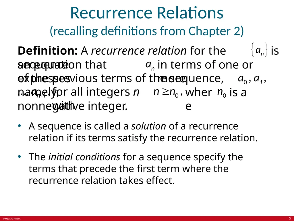
slide5. Recurrence Relations (recalling definitions from Chapter 2) Definition: A recurrence relation for the sequence is an equation that expresses in terms of one or more of the previous terms of the sequence, namely, for all integers n with where is a nonnegative integer.
A sequence is called a solution of a recurrence relation if its terms satisfy the recurrence relation.
The initial conditions for a sequence specify the terms that precede the first term where the recurrence relation takes effect. 5<br>
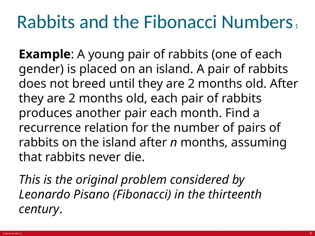
slide6. Rabbits and the Fibonacci Numbers 1 Example: A young pair of rabbits (one of each gender) is placed on an island. A pair of rabbits does not breed until they are 2 months old. After they are 2 months old, each pair of rabbits produces another pair each month. Find a recurrence relation for the number of pairs of rabbits on the island after n months, assuming that rabbits never die.
This is the original problem considered by Leonardo Pisano (Fibonacci) in the thirteenth century. 6<br>
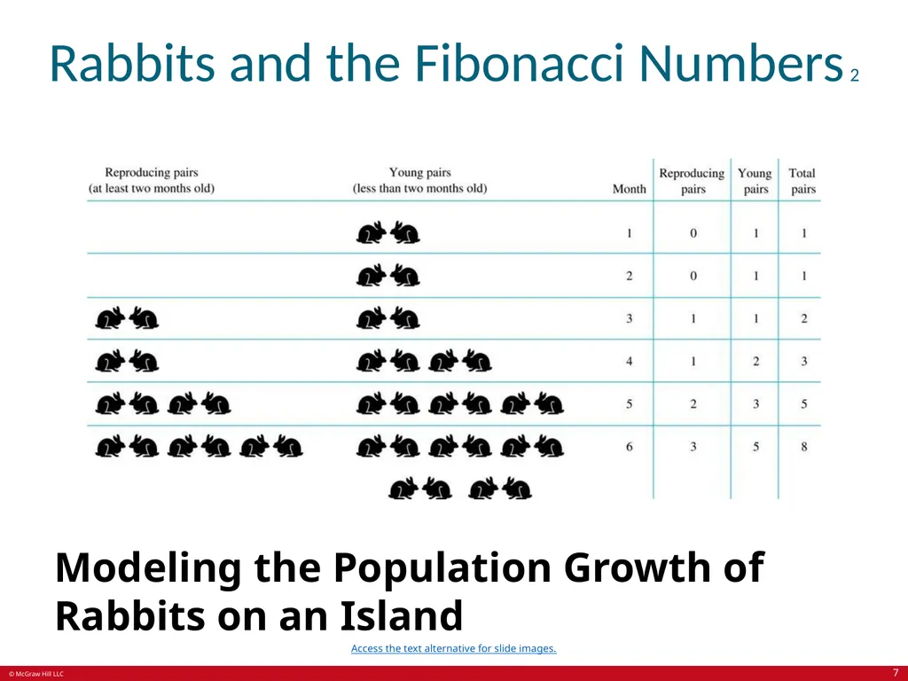
slide7. Rabbits and the Fibonacci Numbers 2 Modeling the Population Growth of Rabbits on an Island Access the text alternative for slide images. 7<br>
slide8. Rabbits and the Fibonacci Numbers 3 Solution: Let be the number of pairs of rabbits after n months. There are is pairs of rabbits on the island at the end of the first month. We also have because the pair does not breed during the first month. To find the number of pairs on the island after n months, add the number on the island after the previous month, and the number of newborn pairs, which equals because each newborn pair comes from a pair at least two months old.
Consequently the sequence satisfies the recurrence relation for n ≥ 3 with the initial conditions The number of pairs of rabbits on the island after n months is given by the nth Fibonacci number. 8<br>
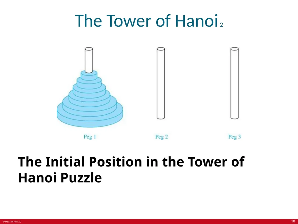
slide9. The Tower of Hanoi 1 In the late nineteenth century, the French mathematician Édouard Lucas invented a puzzle consisting of three pegs on a board with disks of different sizes. Initially all of the disks are on the first peg in order of size, with the largest on the bottom. Rules: You are allowed to move the disks one at a time from one peg to another as long as a larger disk is never placed on a smaller.
Goal: Using allowable moves, end up with all the disks on the second peg in order of size with largest on the bottom. 9<br>
slide10. The Tower of Hanoi 2 The Initial Position in the Tower of Hanoi Puzzle 10<br>
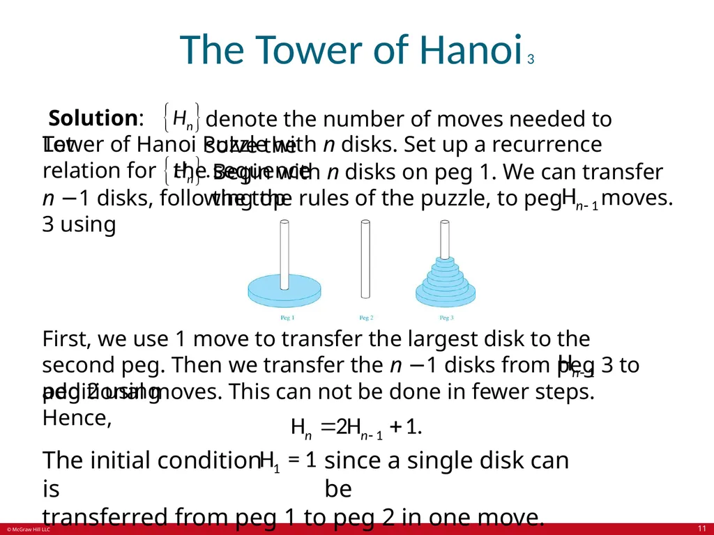
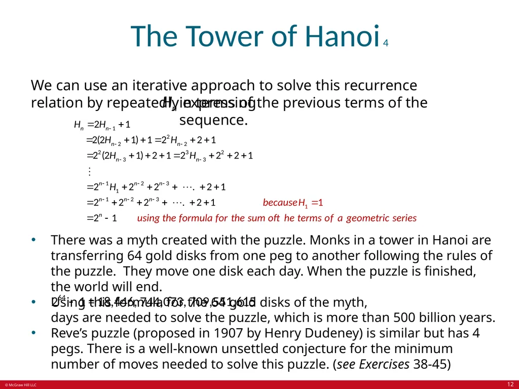
slide11. The Tower of Hanoi 3 Solution: Let denote the number of moves needed to solve the Tower of Hanoi Puzzle with n disks. Set up a recurrence relation for the sequence Begin with n disks on peg 1. We can transfer the top n −1 disks, following the rules of the puzzle, to peg 3 using moves. First, we use 1 move to transfer the largest disk to the second peg. Then we transfer the n −1 disks from peg 3 to peg 2 using additional moves. This can not be done in fewer steps. Hence, The initial condition is since a single disk can be
transferred from peg 1 to peg 2 in one move. 11<br>
slide12. The Tower of Hanoi 4 We can use an iterative approach to solve this recurrence relation by repeatedly expressing in terms of the previous terms of the sequence. There was a myth created with the puzzle. Monks in a tower in Hanoi are transferring 64 gold disks from one peg to another following the rules of the puzzle. They move one disk each day. When the puzzle is finished, the world will end.
Using this formula for the 64 gold disks of the myth, days are needed to solve the puzzle, which is more than 500 billion years.
Reve’s puzzle (proposed in 1907 by Henry Dudeney) is similar but has 4 pegs. There is a well-known unsettled conjecture for the minimum number of moves needed to solve this puzzle. (see Exercises 38-45) 12<br>
slide13. Counting Bit Strings 1 Example 3: Find a recurrence relation and give initial conditions for the number of bit strings of length n without two consecutive 0s. How many such bit strings are there of length five?
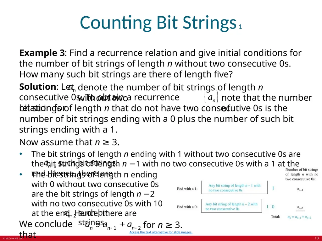
Solution: Let denote the number of bit strings of length n without two consecutive 0s. To obtain a recurrence relation for note that the number of bit strings of length n that do not have two consecutive 0s is the number of bit strings ending with a 0 plus the number of such bit strings ending with a 1.
Now assume that n ≥ 3.
The bit strings of length n ending with 1 without two consecutive 0s are the bit strings of length n −1 with no two consecutive 0s with a 1 at the end. Hence, there are such bit strings. The bit strings of length n ending with 0 without two consecutive 0s are the bit strings of length n −2 with no two consecutive 0s with 10 at the end. Hence, there are such bit strings. We conclude that for n ≥ 3. Access the text alternative for slide images. 13<br>
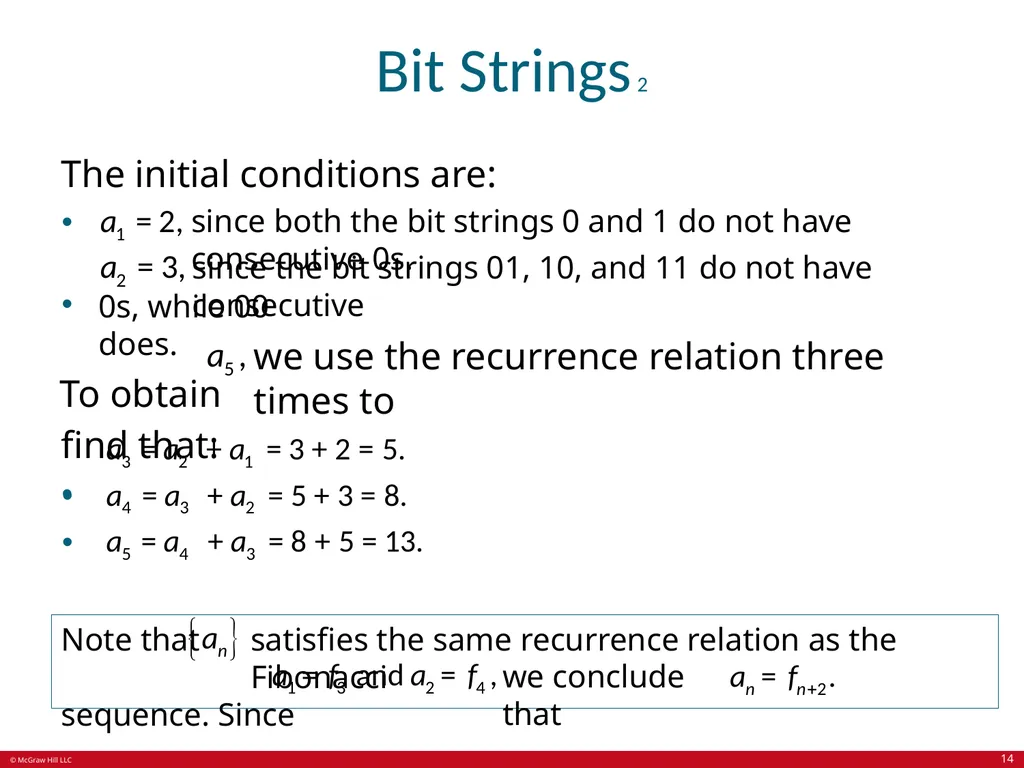
slide14. Bit Strings 2 The initial conditions are: since both the bit strings 0 and 1 do not have consecutive 0s. since the bit strings 01, 10, and 11 do not have consecutive 0s, while 00 does.
To obtain we use the recurrence relation three times to
find that: Note that satisfies the same recurrence relation as the Fibonacci
sequence. Since we conclude that 14<br>
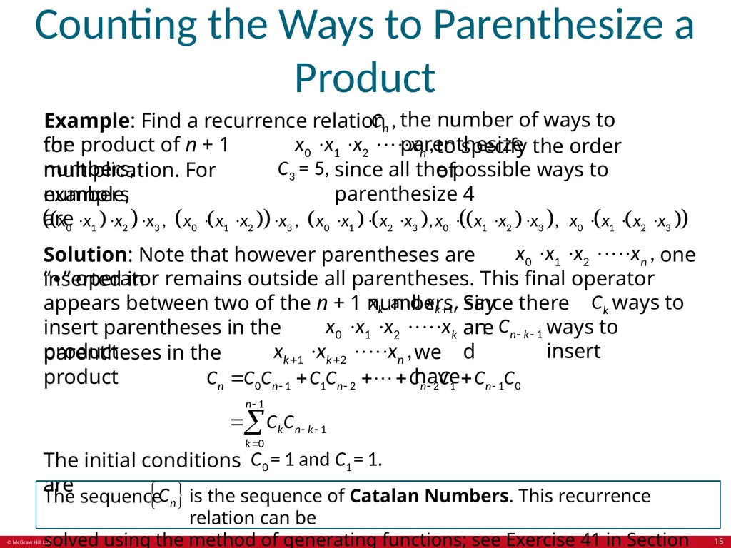
slide15. Counting the Ways to Parenthesize a Product Example: Find a recurrence relation for the number of ways to parenthesize the product of n + 1 numbers, to specify the order of multiplication. For example, since all the possible ways to parenthesize 4 numbers are Solution: Note that however parentheses are inserted in one “∙” operator remains outside all parentheses. This final operator appears between two of the n + 1 numbers, say Since there are ways to insert parentheses in the product and ways to insert parentheses in the product we have The initial conditions are The sequence is the sequence of Catalan Numbers. This recurrence relation can be
solved using the method of generating functions; see Exercise 41 in Section 8.4. 15<br>
slide16. Solving Linear Recurrence Relations Section 8.2 16<br>
slide17. Section Summary 2 Linear Homogeneous Recurrence Relations.
Solving Linear Homogeneous Recurrence Relations with Constant Coefficients.
Solving Linear Nonhomogeneous Recurrence Relations with Constant Coefficients. 17<br>
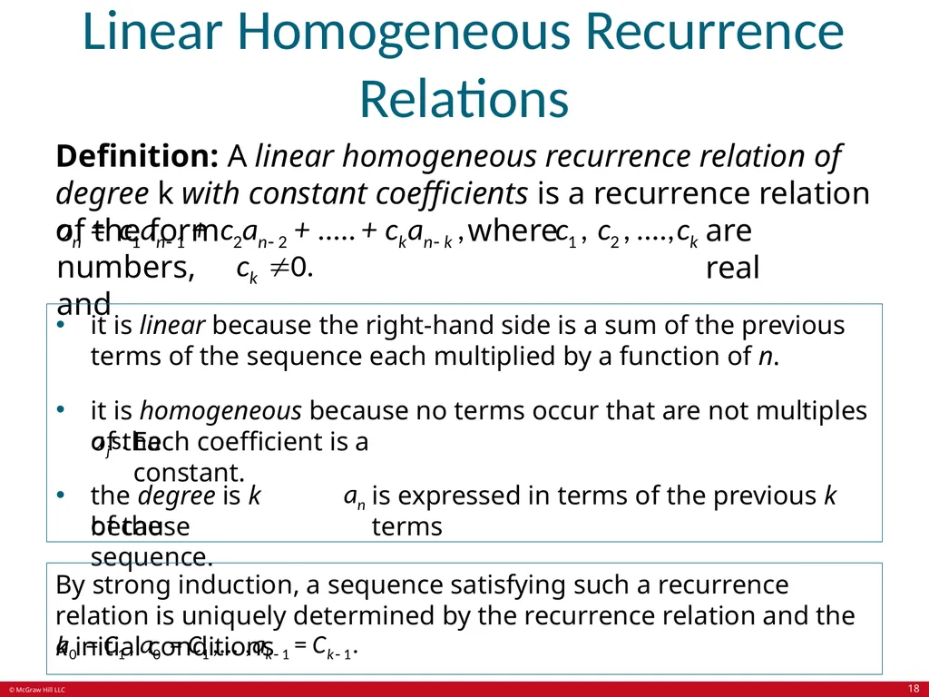
slide18. Linear Homogeneous Recurrence Relations Definition: A linear homogeneous recurrence relation of degree k with constant coefficients is a recurrence relation of the form where are real numbers, and it is linear because the right-hand side is a sum of the previous terms of the sequence each multiplied by a function of n.
it is homogeneous because no terms occur that are not multiples of the Each coefficient is a constant. the degree is k because is expressed in terms of the previous k terms of the sequence. By strong induction, a sequence satisfying such a recurrence relation is uniquely determined by the recurrence relation and the k initial conditions 18<br>
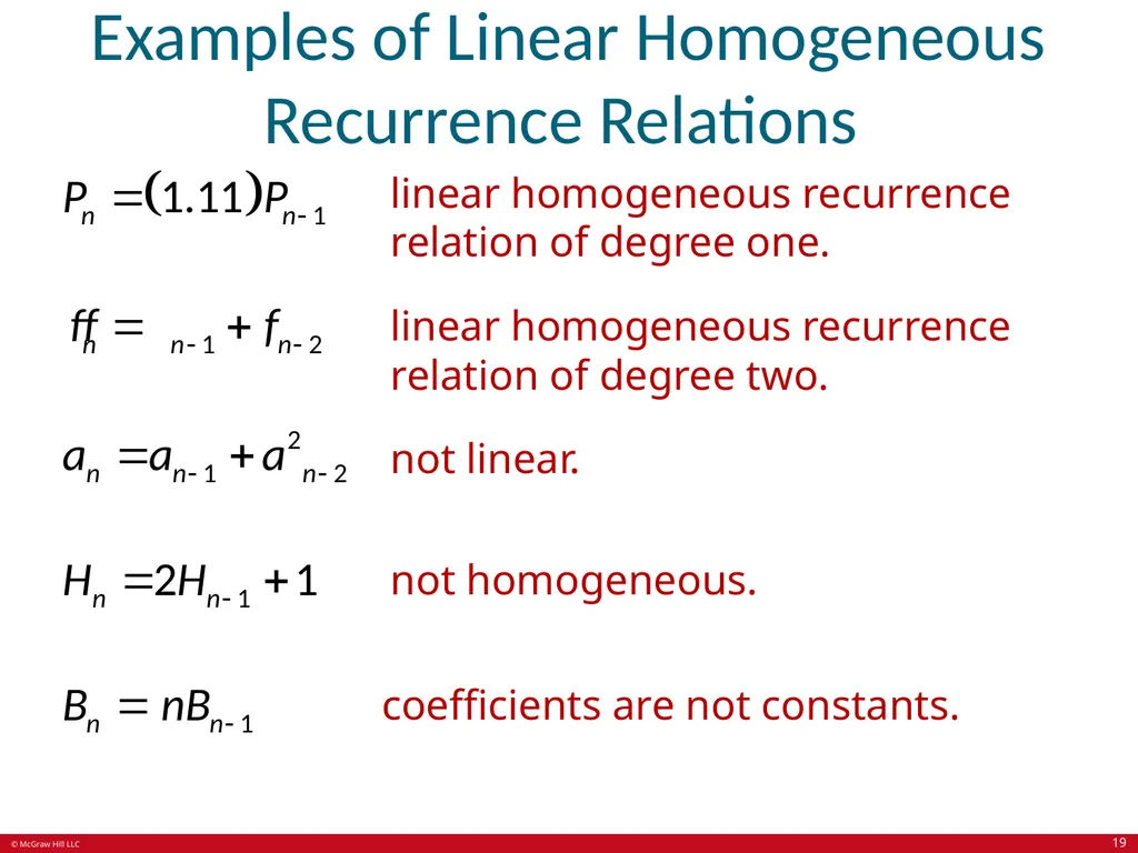
slide19. Examples of Linear Homogeneous Recurrence Relations linear homogeneous recurrence relation of degree one. linear homogeneous recurrence relation of degree two. not linear. not homogeneous. coefficients are not constants. 19<br>
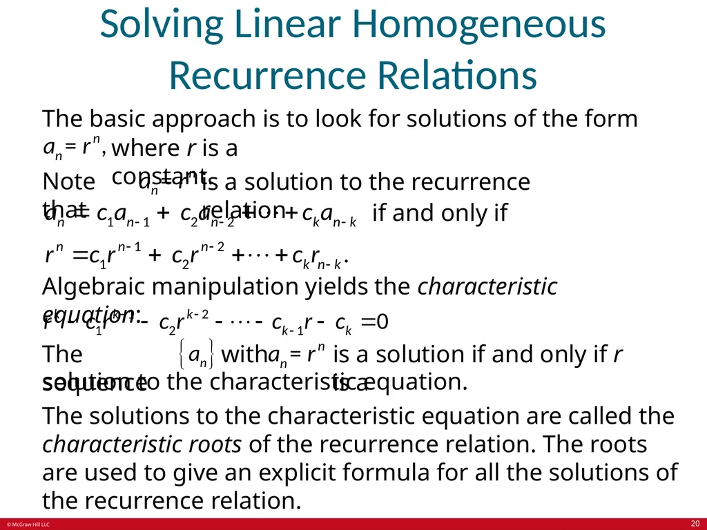
slide20. Solving Linear Homogeneous Recurrence Relations The basic approach is to look for solutions of the form where r is a constant. Note that is a solution to the recurrence relation if and only if Algebraic manipulation yields the characteristic equation: The sequence with is a solution if and only if r is a solution to the characteristic equation.
The solutions to the characteristic equation are called the characteristic roots of the recurrence relation. The roots are used to give an explicit formula for all the solutions of the recurrence relation. 20<br>
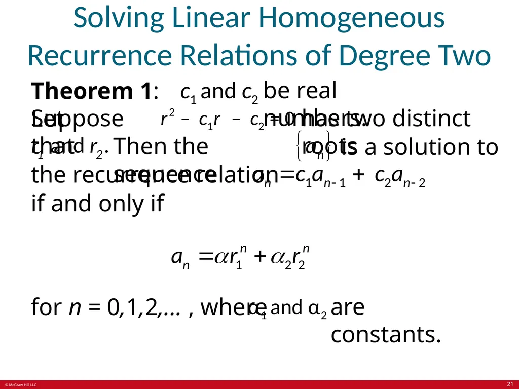
slide21. Solving Linear Homogeneous Recurrence Relations of Degree Two Theorem 1: Let be real numbers. Suppose that has two distinct roots Then the sequence is a solution to
the recurrence relation if and only if for n = 0,1,2, . . . , where are constants. 21<br>
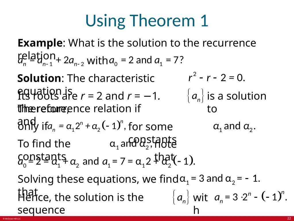
slide22. Using Theorem 1 Example: What is the solution to the recurrence relation with Solution: The characteristic equation is Its roots are r = 2 and r = −1. Therefore, is a solution to the recurrence relation if and only if for some constants To find the constants note that Solving these equations, we find that Hence, the solution is the sequence with 22<br>
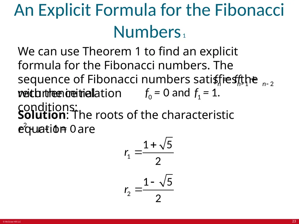
slide23. An Explicit Formula for the Fibonacci Numbers 1 We can use Theorem 1 to find an explicit formula for the Fibonacci numbers. The sequence of Fibonacci numbers satisfies the recurrence relation with the initial conditions: Solution: The roots of the characteristic equation are 23<br>
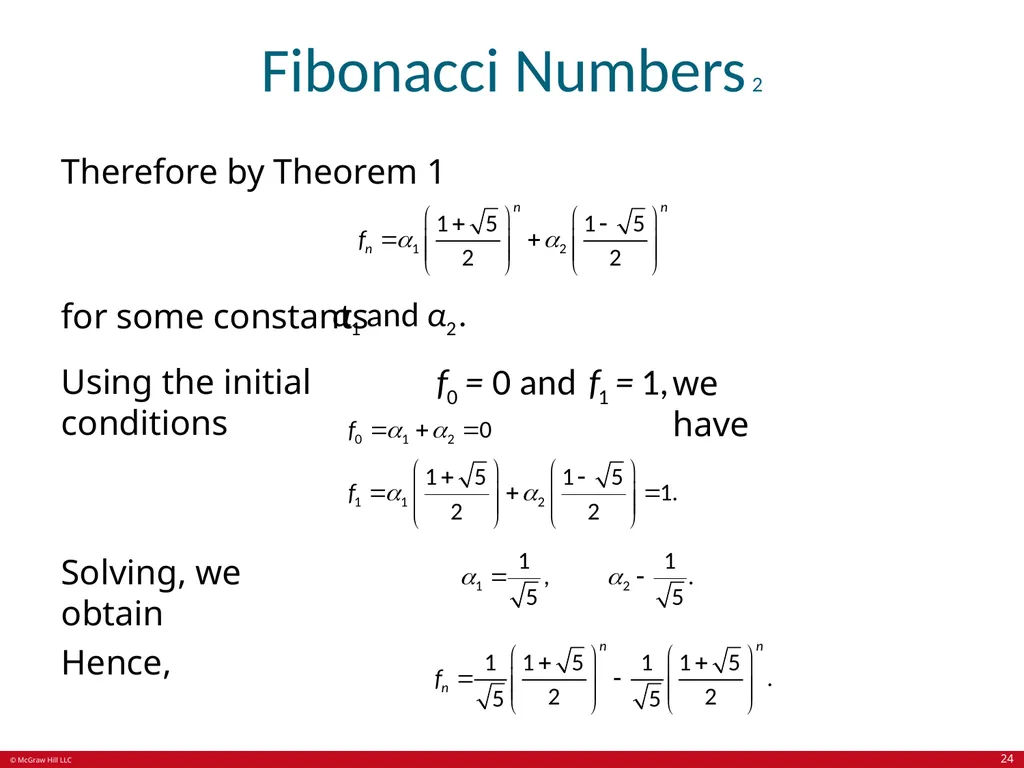
slide24. Fibonacci Numbers 2 Therefore by Theorem 1 for some constants Using the initial conditions we have Solving, we obtain Hence, 24<br>
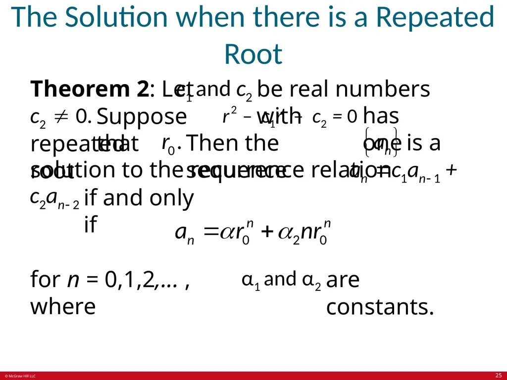
slide25. The Solution when there is a Repeated Root Theorem 2: Let be real numbers with Suppose that has one repeated root Then the sequence is a
solution to the recurrence relation if and only if for n = 0,1,2, . . . , where are constants. 25<br>
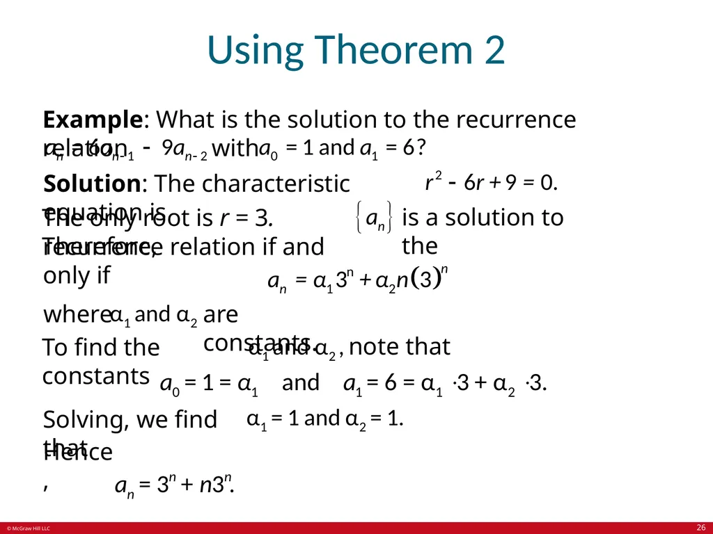
slide26. Using Theorem 2 Example: What is the solution to the recurrence relation with Solution: The characteristic equation is The only root is r = 3. Therefore, is a solution to the recurrence relation if and only if where are constants. To find the constants note that Solving, we find that Hence, 26<br>
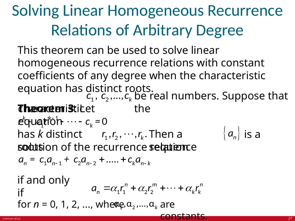
slide27. Solving Linear Homogeneous Recurrence Relations of Arbitrary Degree This theorem can be used to solve linear homogeneous recurrence relations with constant coefficients of any degree when the characteristic equation has distinct roots.
Theorem 3: Let be real numbers. Suppose that the characteristic equation has k distinct roots Then a sequence is a
solution of the recurrence relation if and only if for n = 0, 1, 2, . . . , where are constants. 27<br>
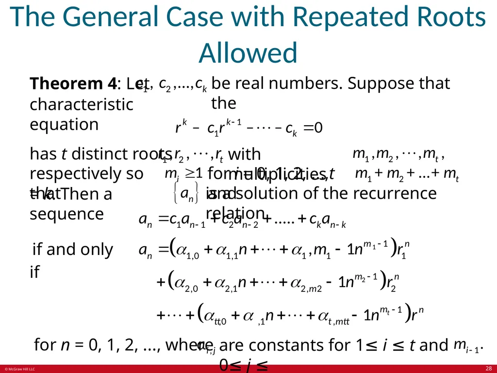
slide28. The General Case with Repeated Roots Allowed Theorem 4: Let be real numbers. Suppose that the characteristic equation has t distinct roots with multiplicities respectively so that for i = 0, 1, 2, . . . ,t and = k. Then a sequence is a solution of the recurrence relation if and only if for n = 0, 1, 2, . . . , where are constants for 1≤ i ≤ t and 0≤ j ≤ 28<br>
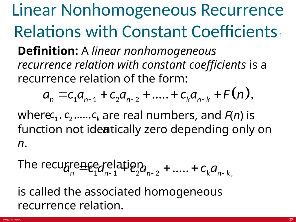
slide29. Linear Nonhomogeneous Recurrence Relations with Constant Coefficients 1 Definition: A linear nonhomogeneous recurrence relation with constant coefficients is a recurrence relation of the form: where are real numbers, and F(n) is a function not identically zero depending only on n.
The recurrence relation is called the associated homogeneous recurrence relation. 29<br>
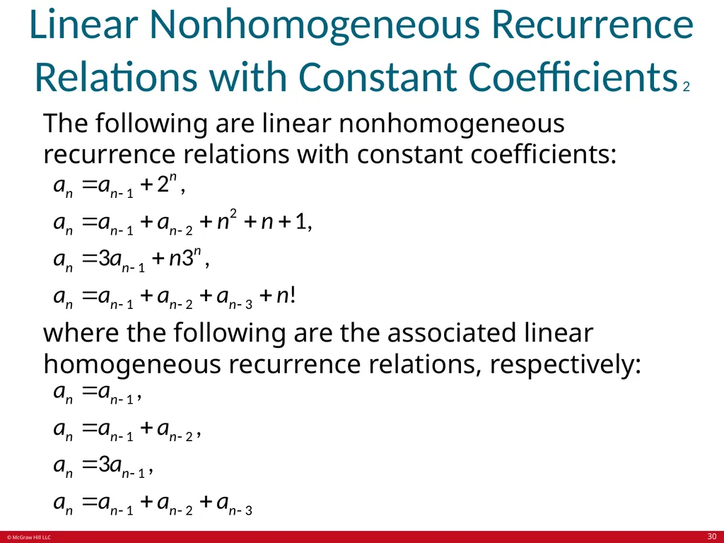
slide30. Linear Nonhomogeneous Recurrence Relations with Constant Coefficients 2 The following are linear nonhomogeneous recurrence relations with constant coefficients: where the following are the associated linear homogeneous recurrence relations, respectively: 30<br>
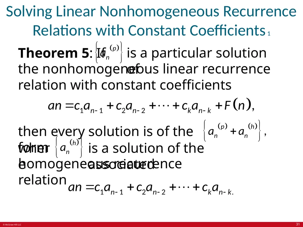
slide31. Solving Linear Nonhomogeneous Recurrence Relations with Constant Coefficients 1 Theorem 5: If is a particular solution of the nonhomogeneous linear recurrence relation with constant coefficients then every solution is of the form where is a solution of the associated homogeneous recurrence relation 31<br>
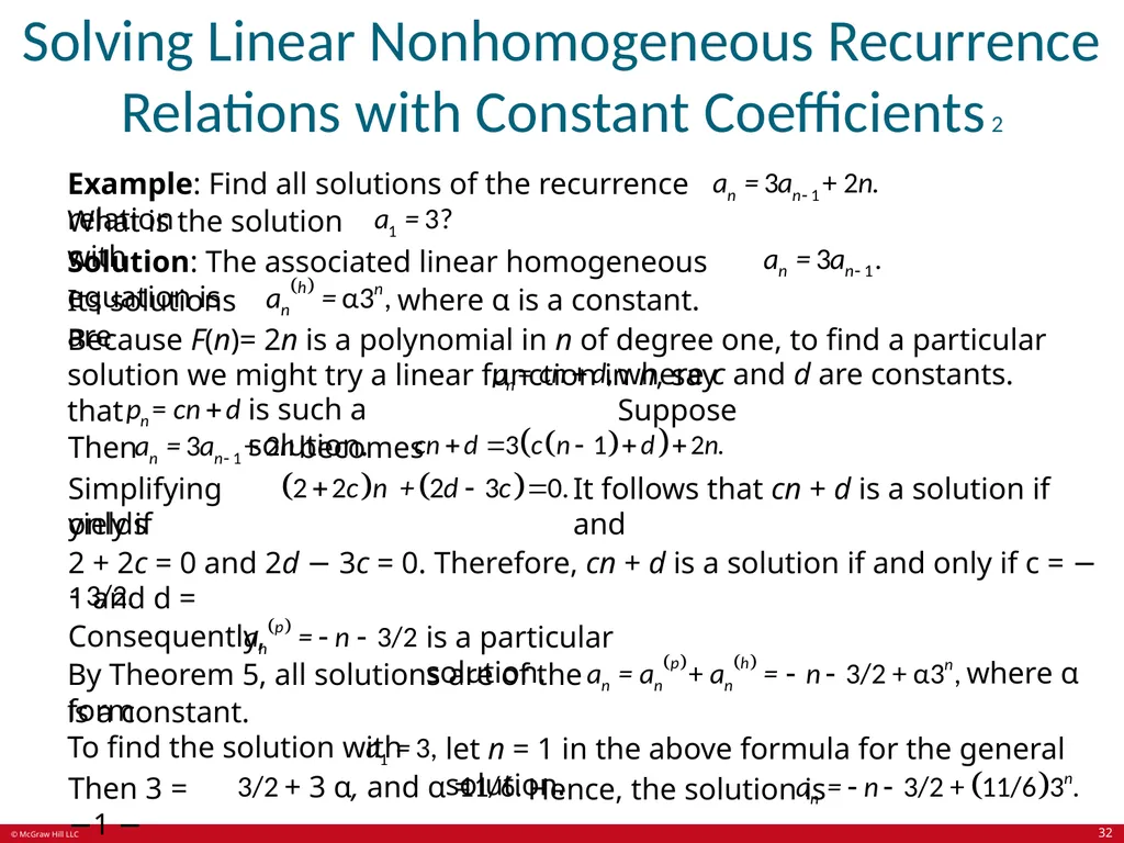
slide32. Solving Linear Nonhomogeneous Recurrence Relations with Constant Coefficients 2 Example: Find all solutions of the recurrence relation What is the solution with Solution: The associated linear homogeneous equation is Its solutions are where α is a constant. Because F(n)= 2n is a polynomial in n of degree one, to find a particular solution we might try a linear function in n, say where c and d are constants. Suppose that is such a solution. Then becomes Simplifying yields It follows that cn + d is a solution if and only if
2 + 2c = 0 and 2d − 3c = 0. Therefore, cn + d is a solution if and only if c = − 1 and d = Consequently, is a particular solution. By Theorem 5, all solutions are of the form where α
is a constant.
To find the solution with let n = 1 in the above formula for the general solution. Then 3 = −1 − + 3 α, and α = Hence, the solution is 32<br>
slide33. Divide-and-Conquer Algorithms and Recurrence Relations Section 8.3 33<br>
slide34. Section Summary 3 Divide-and-Conquer Algorithms and Recurrence Relations.
Examples.
Binary Search.
Merge Sort.
Fast Multiplication of Integers.
Master Theorem.
Closest Pair of Points (not covered yet in these slides). 34<br>
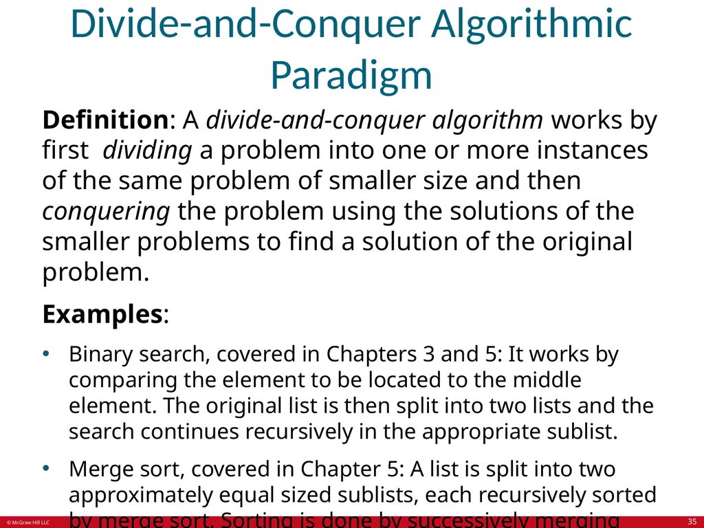
slide35. Divide-and-Conquer Algorithmic Paradigm Definition: A divide-and-conquer algorithm works by first dividing a problem into one or more instances of the same problem of smaller size and then conquering the problem using the solutions of the smaller problems to find a solution of the original problem.
Examples:
Binary search, covered in Chapters 3 and 5: It works by comparing the element to be located to the middle element. The original list is then split into two lists and the search continues recursively in the appropriate sublist.
Merge sort, covered in Chapter 5: A list is split into two approximately equal sized sublists, each recursively sorted by merge sort. Sorting is done by successively merging pairs of lists. 35<br>
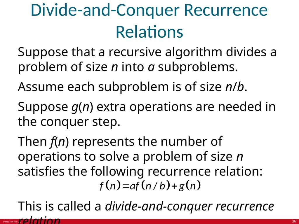
slide36. Divide-and-Conquer Recurrence Relations Suppose that a recursive algorithm divides a problem of size n into a subproblems.
Assume each subproblem is of size n/b.
Suppose g(n) extra operations are needed in the conquer step.
Then f(n) represents the number of operations to solve a problem of size n satisfies the following recurrence relation: This is called a divide-and-conquer recurrence relation. 36<br>
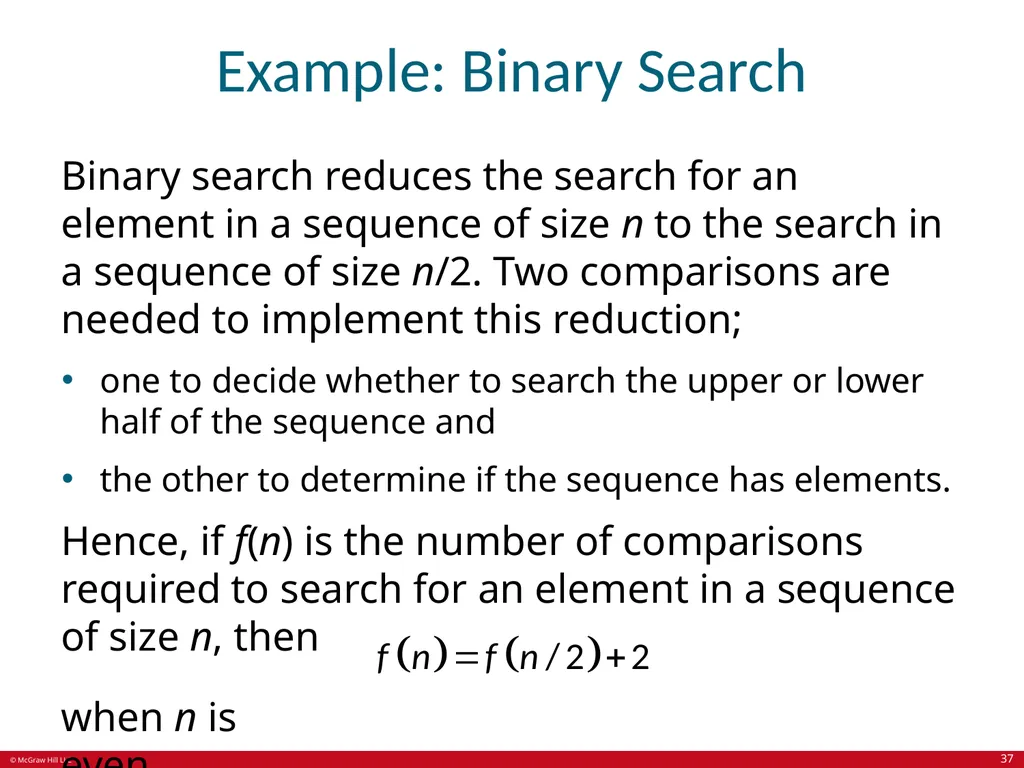
slide37. Example: Binary Search Binary search reduces the search for an element in a sequence of size n to the search in a sequence of size n/2. Two comparisons are needed to implement this reduction;
one to decide whether to search the upper or lower half of the sequence and
the other to determine if the sequence has elements.
Hence, if f(n) is the number of comparisons required to search for an element in a sequence of size n, then when n is even. 37<br>
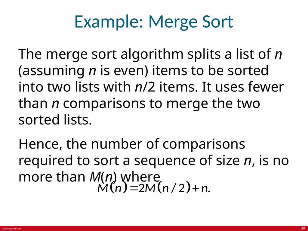
slide38. Example: Merge Sort The merge sort algorithm splits a list of n (assuming n is even) items to be sorted into two lists with n/2 items. It uses fewer than n comparisons to merge the two sorted lists.
Hence, the number of comparisons required to sort a sequence of size n, is no more than M(n) where 38<br>
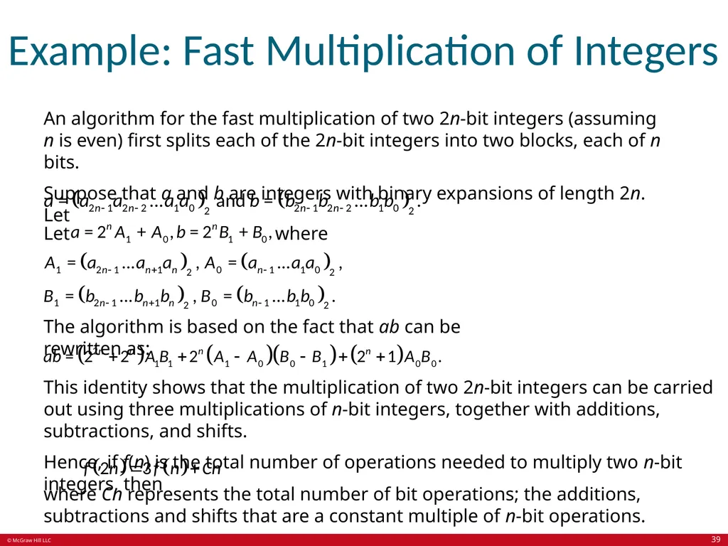
slide39. Example: Fast Multiplication of Integers An algorithm for the fast multiplication of two 2n-bit integers (assuming n is even) first splits each of the 2n-bit integers into two blocks, each of n bits.
Suppose that a and b are integers with binary expansions of length 2n. Let Let where The algorithm is based on the fact that ab can be rewritten as: This identity shows that the multiplication of two 2n-bit integers can be carried out using three multiplications of n-bit integers, together with additions, subtractions, and shifts.
Hence, if f(n) is the total number of operations needed to multiply two n-bit integers, then where Cn represents the total number of bit operations; the additions, subtractions and shifts that are a constant multiple of n-bit operations. 39<br>
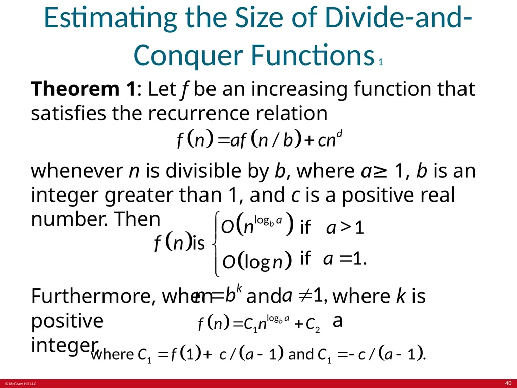
slide40. Estimating the Size of Divide-and-Conquer Functions 1 Theorem 1: Let f be an increasing function that satisfies the recurrence relation whenever n is divisible by b, where a≥ 1, b is an integer greater than 1, and c is a positive real number. Then Furthermore, when and where k is a positive integer, 40<br>
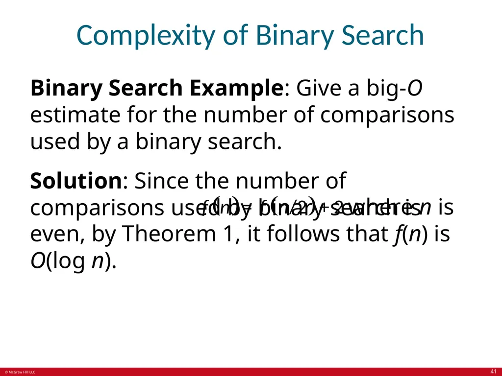
slide41. Complexity of Binary Search Binary Search Example: Give a big-O estimate for the number of comparisons used by a binary search.
Solution: Since the number of comparisons used by binary search is where n is even, by Theorem 1, it follows that f(n) is O(log n). 41<br>
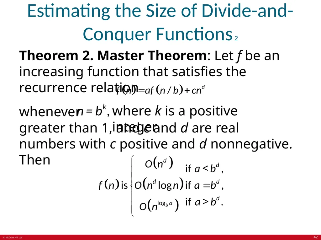
slide42. Estimating the Size of Divide-and-Conquer Functions 2 Theorem 2. Master Theorem: Let f be an increasing function that satisfies the recurrence relation whenever where k is a positive integer greater than 1, and c and d are real numbers with c positive and d nonnegative. Then 42<br>
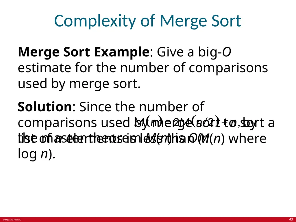
slide43. Complexity of Merge Sort Merge Sort Example: Give a big-O estimate for the number of comparisons used by merge sort.
Solution: Since the number of comparisons used by merge sort to sort a list of n elements is less than M(n) where by the master theorem M(n) is O(n log n). 43<br>
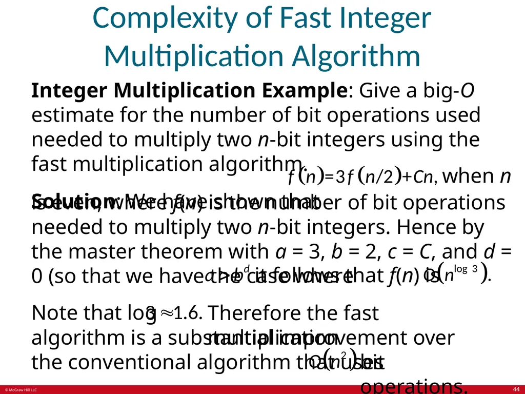
slide44. Complexity of Fast Integer Multiplication Algorithm Integer Multiplication Example: Give a big-O estimate for the number of bit operations used needed to multiply two n-bit integers using the fast multiplication algorithm.
Solution: We have shown that when n is even, where f(n) is the number of bit operations needed to multiply two n-bit integers. Hence by the master theorem with a = 3, b = 2, c = C, and d = 0 (so that we have the case where it follows that f(n) is Note that log Therefore the fast multiplication algorithm is a substantial improvement over the conventional algorithm that uses bit operations. 44<br>
slide45. Generating Functions Section 8.4 45<br>
slide46. Section Summary 4 Generating Functions.
Counting Problems and Generating Functions.
Useful Generating Functions.
Solving Recurrence Relations Using Generating Functions (not yet covered in the slides).
Proving Identities Using Generating Functions (not yet covered in the slides). 46<br>
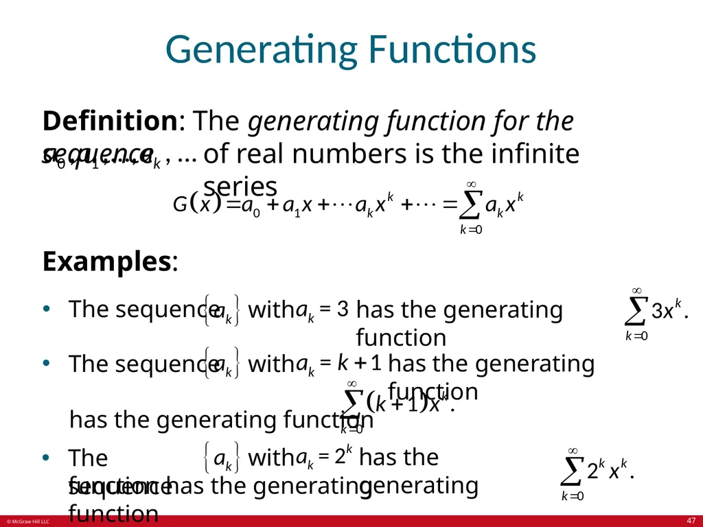
slide47. Generating Functions Definition: The generating function for the sequence of real numbers is the infinite series Examples:
The sequence with has the generating function The sequence with has the generating function
has the generating function The sequence with has the generating function has the generating function 47<br>
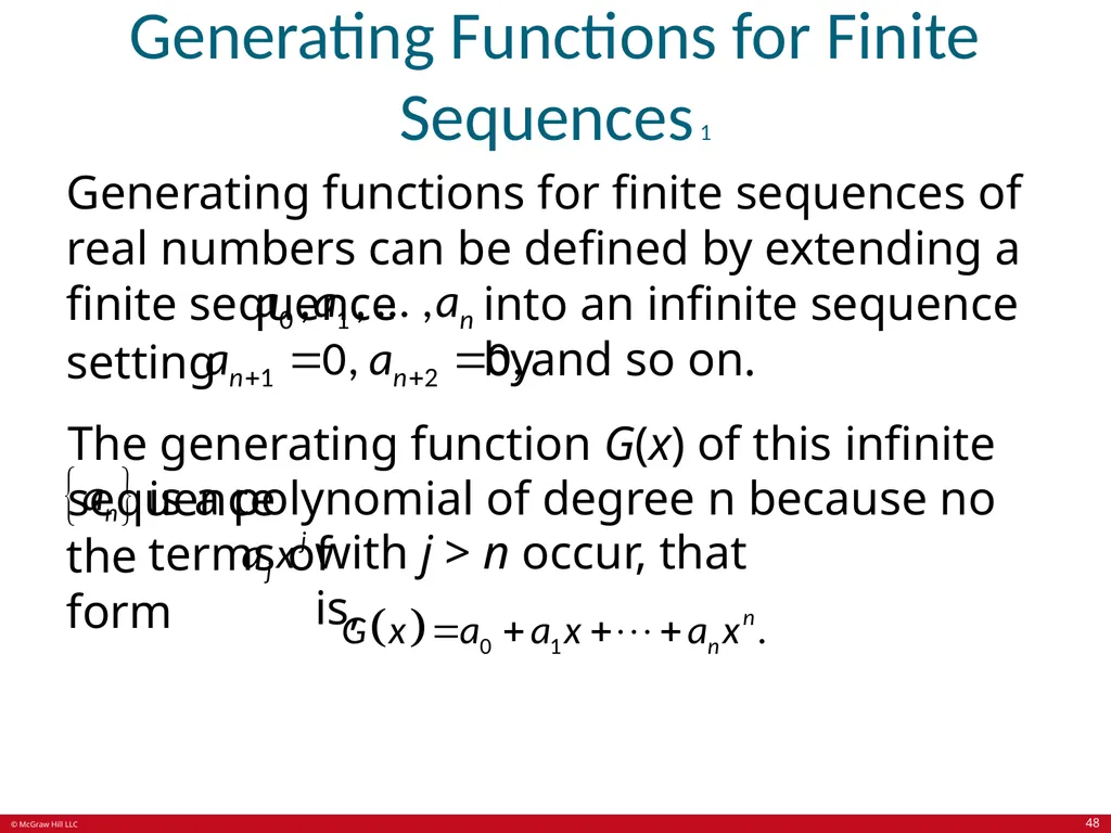
slide48. Generating Functions for Finite Sequences 1 Generating functions for finite sequences of real numbers can be defined by extending a finite sequence into an infinite sequence by setting and so on. The generating function G(x) of this infinite sequence is a polynomial of degree n because no terms of the form with j > n occur, that is, 48<br>
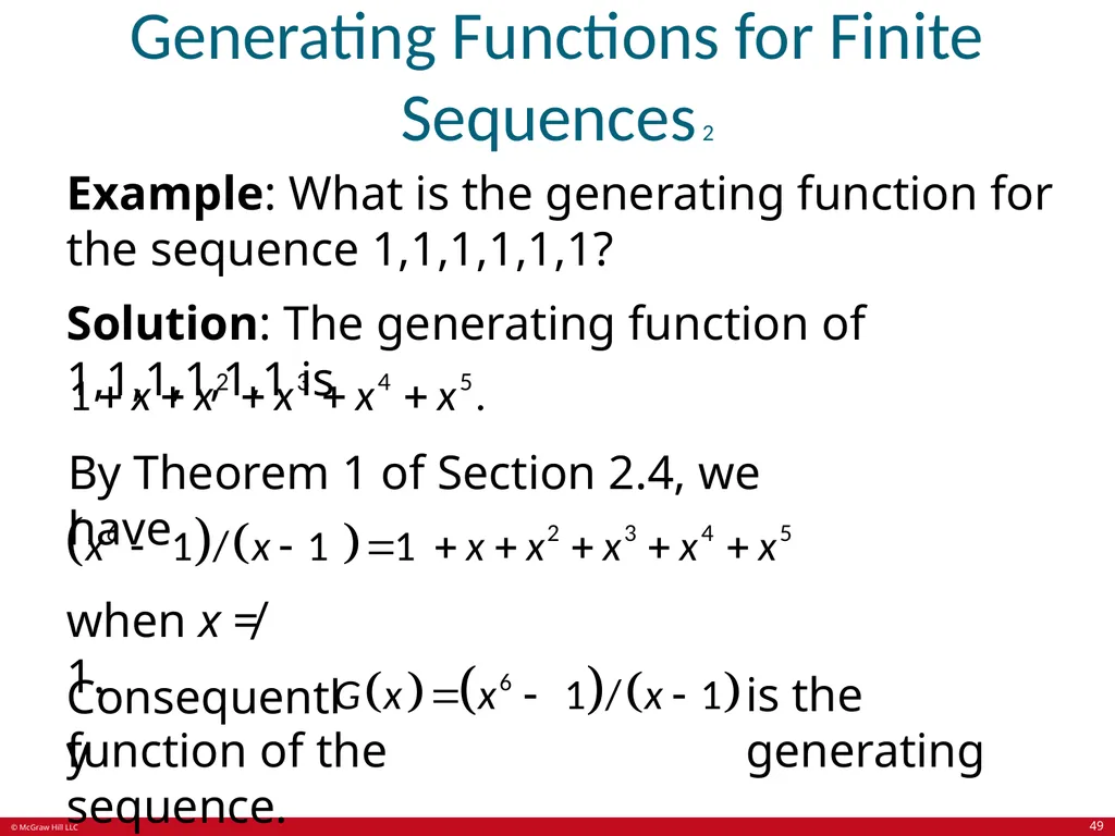
slide49. Generating Functions for Finite Sequences 2 Example: What is the generating function for the sequence 1,1,1,1,1,1?
Solution: The generating function of 1,1,1,1,1,1 is By Theorem 1 of Section 2.4, we have when x ≠ 1. Consequently is the generating function of the sequence. 49<br>
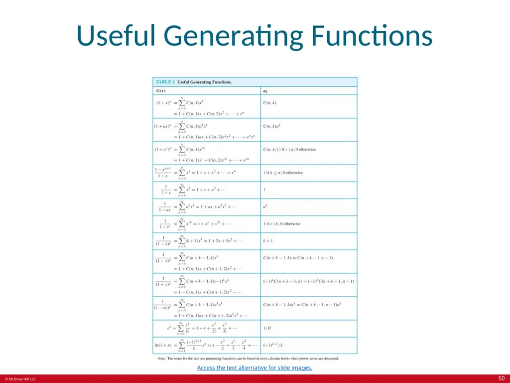
slide50. Useful Generating Functions Access the text alternative for slide images. 50<br>
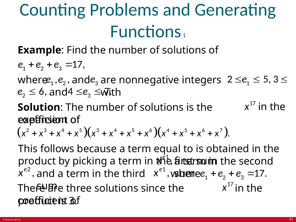
slide51. Counting Problems and Generating Functions 1 Example: Find the number of solutions of where and are nonnegative integers with and Solution: The number of solutions is the coefficient of in the expansion of This follows because a term equal to is obtained in the product by picking a term in the first sum a term in the second sum and a term in the third sum where There are three solutions since the coefficient of in the product is 3. 51<br>
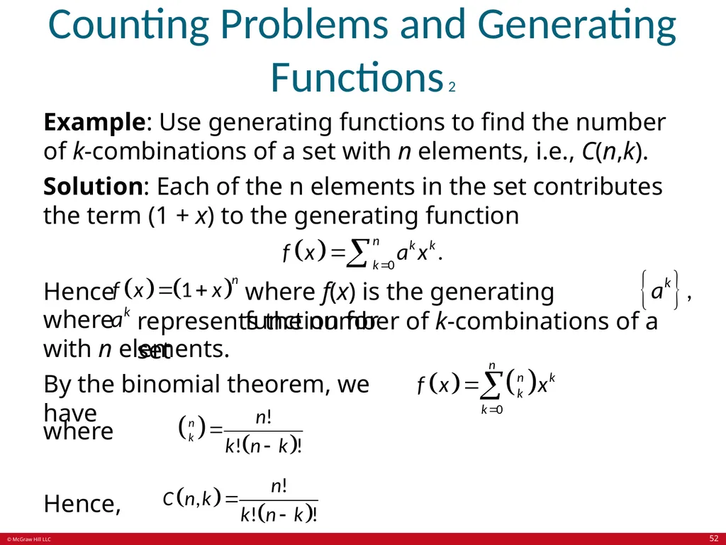
slide52. Counting Problems and Generating Functions 2 Example: Use generating functions to find the number of k-combinations of a set with n elements, i.e., C(n,k).
Solution: Each of the n elements in the set contributes the term (1 + x) to the generating function Hence where f(x) is the generating function for where represents the number of k-combinations of a set with n elements.
By the binomial theorem, we have where Hence, 52<br>
slide53. Inclusion-Exclusion Section 8.5 53<br>
slide54. Section Summary 5 The Principle of Inclusion-Exclusion.
Examples. 54<br>
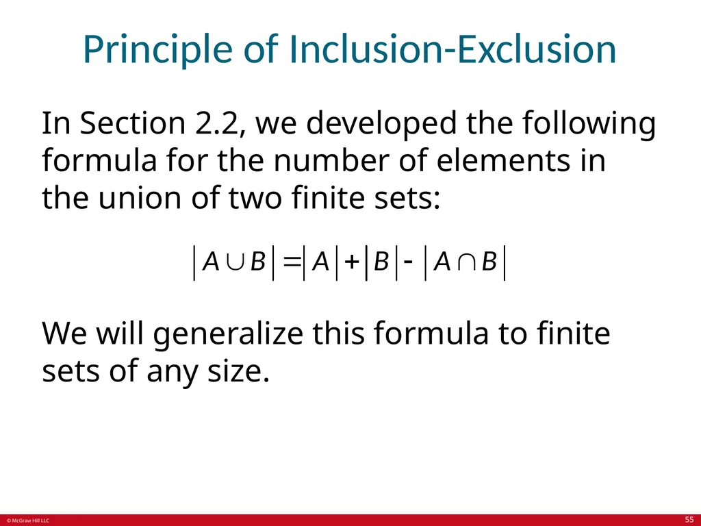
slide55. Principle of Inclusion-Exclusion In Section 2.2, we developed the following formula for the number of elements in the union of two finite sets: We will generalize this formula to finite sets of any size. 55<br>
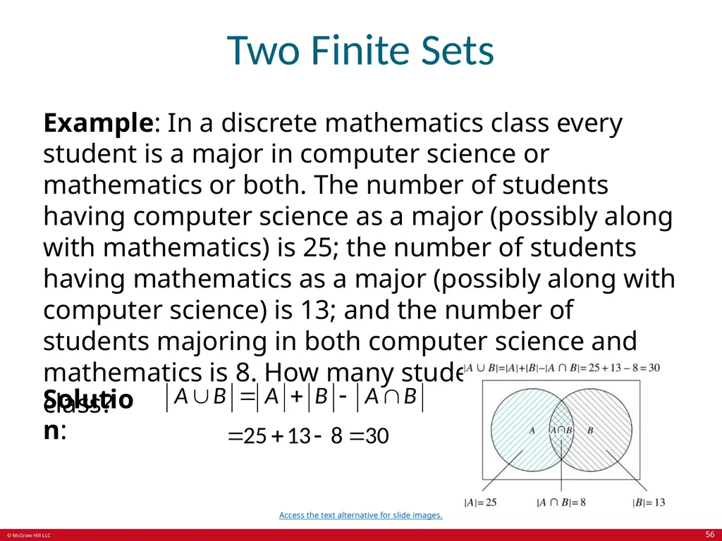
slide56. Two Finite Sets Example: In a discrete mathematics class every student is a major in computer science or mathematics or both. The number of students having computer science as a major (possibly along with mathematics) is 25; the number of students having mathematics as a major (possibly along with computer science) is 13; and the number of students majoring in both computer science and mathematics is 8. How many students are in the class? Solution: Access the text alternative for slide images. 56<br>
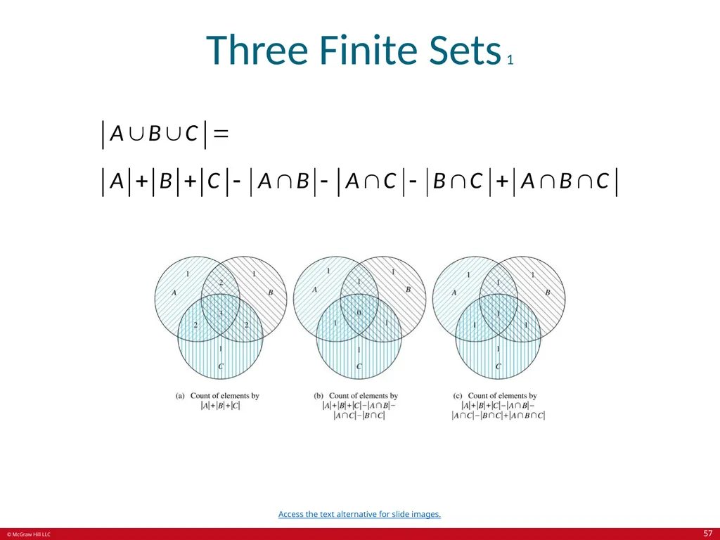
slide57. Three Finite Sets 1 Access the text alternative for slide images. 57<br>
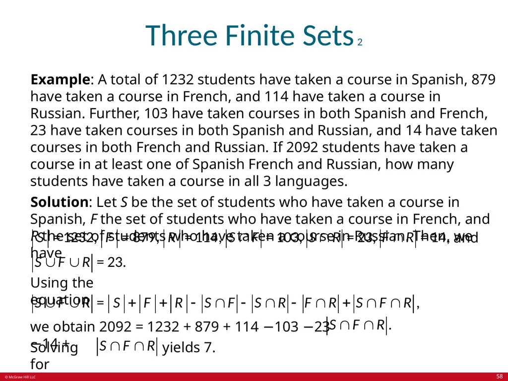
slide58. Three Finite Sets 2 Example: A total of 1232 students have taken a course in Spanish, 879 have taken a course in French, and 114 have taken a course in Russian. Further, 103 have taken courses in both Spanish and French, 23 have taken courses in both Spanish and Russian, and 14 have taken courses in both French and Russian. If 2092 students have taken a course in at least one of Spanish French and Russian, how many students have taken a course in all 3 languages.
Solution: Let S be the set of students who have taken a course in Spanish, F the set of students who have taken a course in French, and R the set of students who have taken a course in Russian. Then, we have and Using the equation we obtain 2092 = 1232 + 879 + 114 −103 −23 −14 + Solving for yields 7. 58<br>
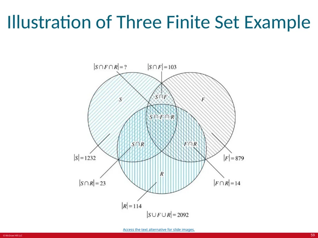
slide59. Illustration of Three Finite Set Example Access the text alternative for slide images. 59<br>
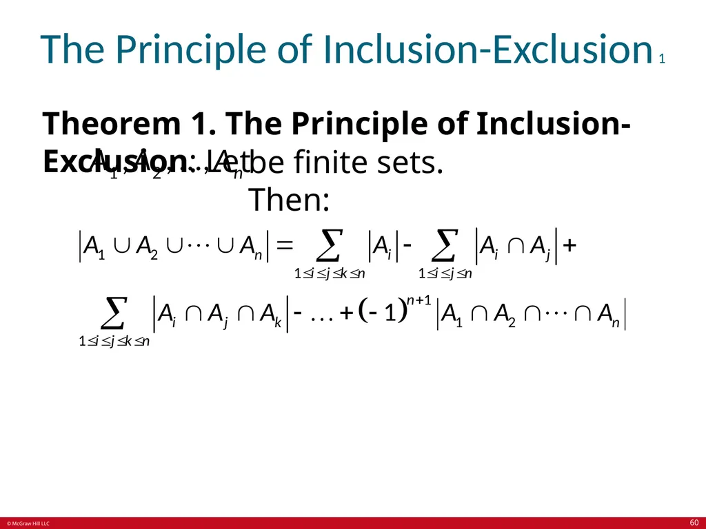
slide60. The Principle of Inclusion-Exclusion 1 Theorem 1. The Principle of Inclusion-Exclusion: Let be finite sets. Then: 60<br>
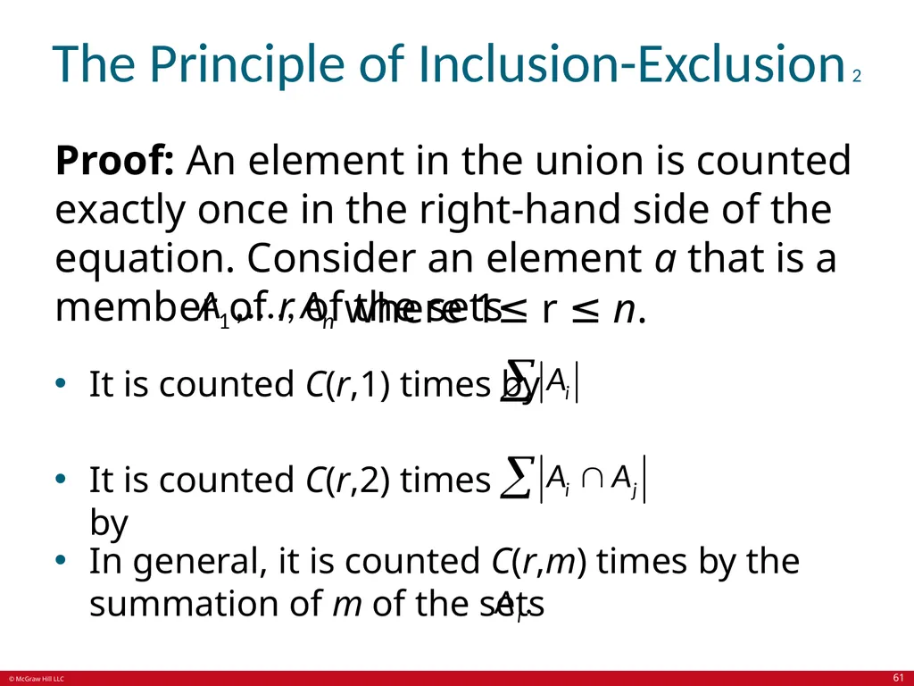
slide61. The Principle of Inclusion-Exclusion 2 Proof: An element in the union is counted exactly once in the right-hand side of the equation. Consider an element a that is a member of r of the sets where 1≤ r ≤ n.
It is counted C(r,1) times by It is counted C(r,2) times by In general, it is counted C(r,m) times by the summation of m of the sets 61<br>
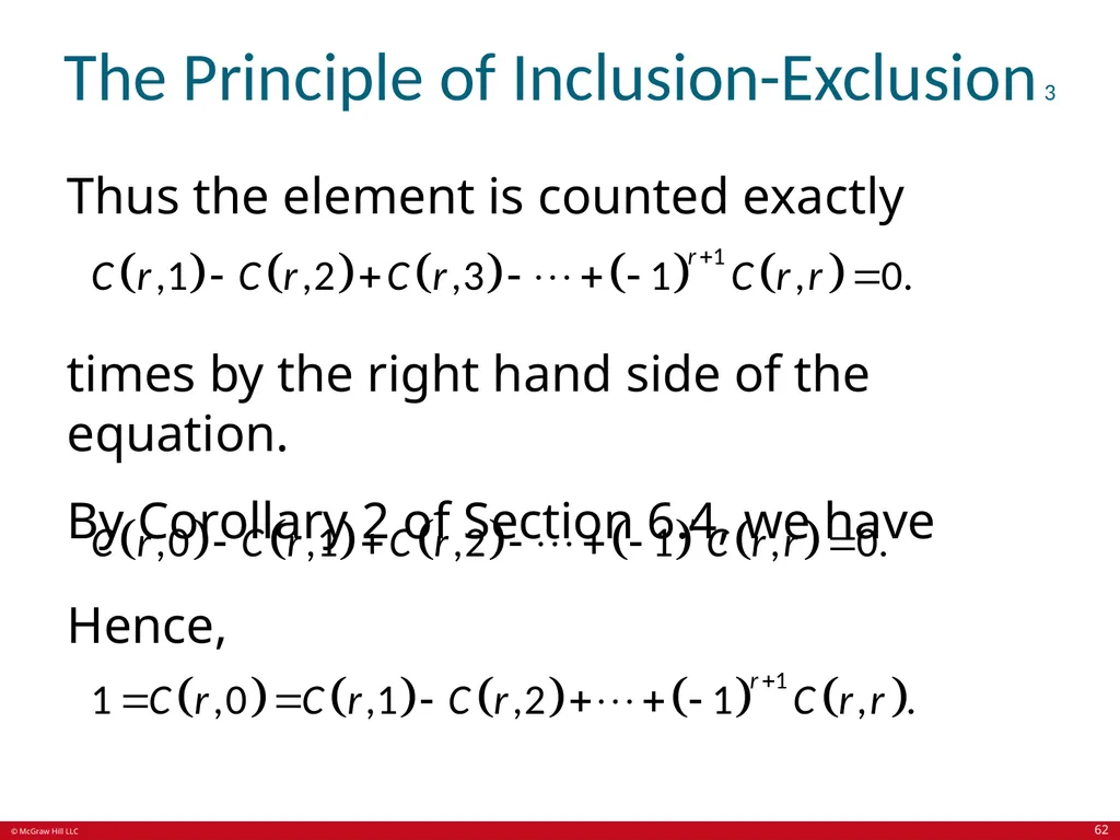
slide62. The Principle of Inclusion-Exclusion 3 Thus the element is counted exactly times by the right hand side of the equation.
By Corollary 2 of Section 6.4, we have Hence, 62<br>
slide63. Applications of Inclusion-Exclusion Section 8.6 63<br>
slide64. Section Summary 6 Counting Onto-Functions.
Derangements. 64<br>
slide65. The Number of Onto Functions 1 Example: How many onto functions are there from a set with six elements to a set with three elements?
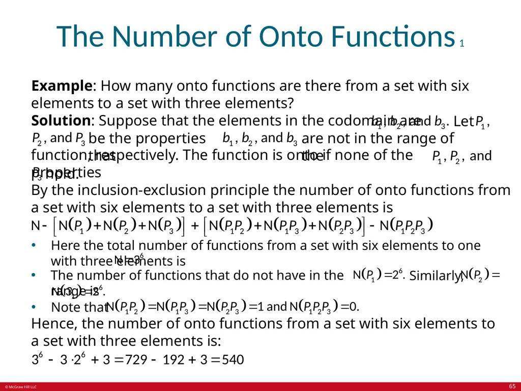
Solution: Suppose that the elements in the codomain are Let be the properties that are not in the range of the function, respectively. The function is onto if none of the properties hold. By the inclusion-exclusion principle the number of onto functions from a set with six elements to a set with three elements is Here the total number of functions from a set with six elements to one with three elements is The number of functions that do not have in the range is Similarly, Note that Hence, the number of onto functions from a set with six elements to a set with three elements is: 65<br>
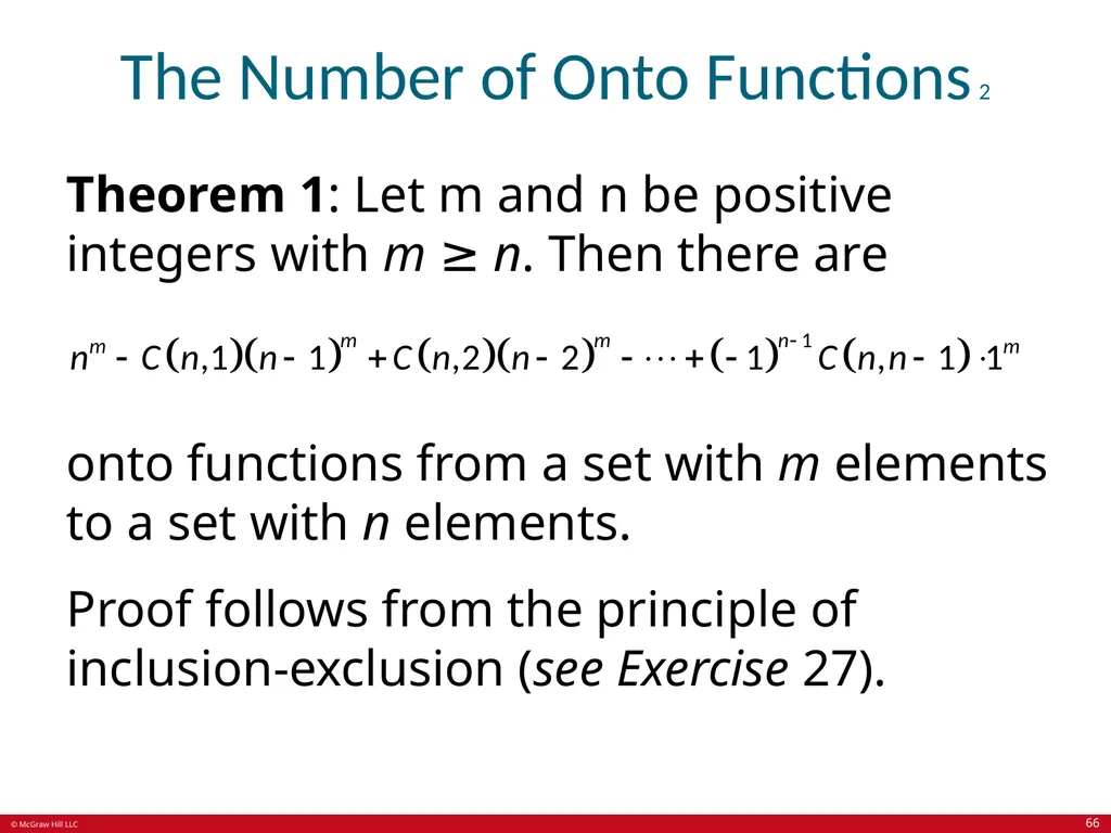
slide66. The Number of Onto Functions 2 Theorem 1: Let m and n be positive integers with m ≥ n. Then there are onto functions from a set with m elements to a set with n elements.
Proof follows from the principle of inclusion-exclusion (see Exercise 27). 66<br>
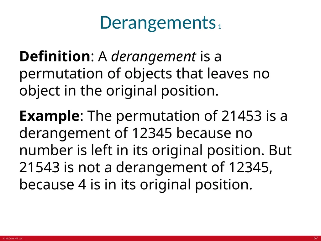
slide67. Derangements 1 Definition: A derangement is a permutation of objects that leaves no object in the original position.
Example: The permutation of 21453 is a derangement of 12345 because no number is left in its original position. But 21543 is not a derangement of 12345, because 4 is in its original position. 67<br>
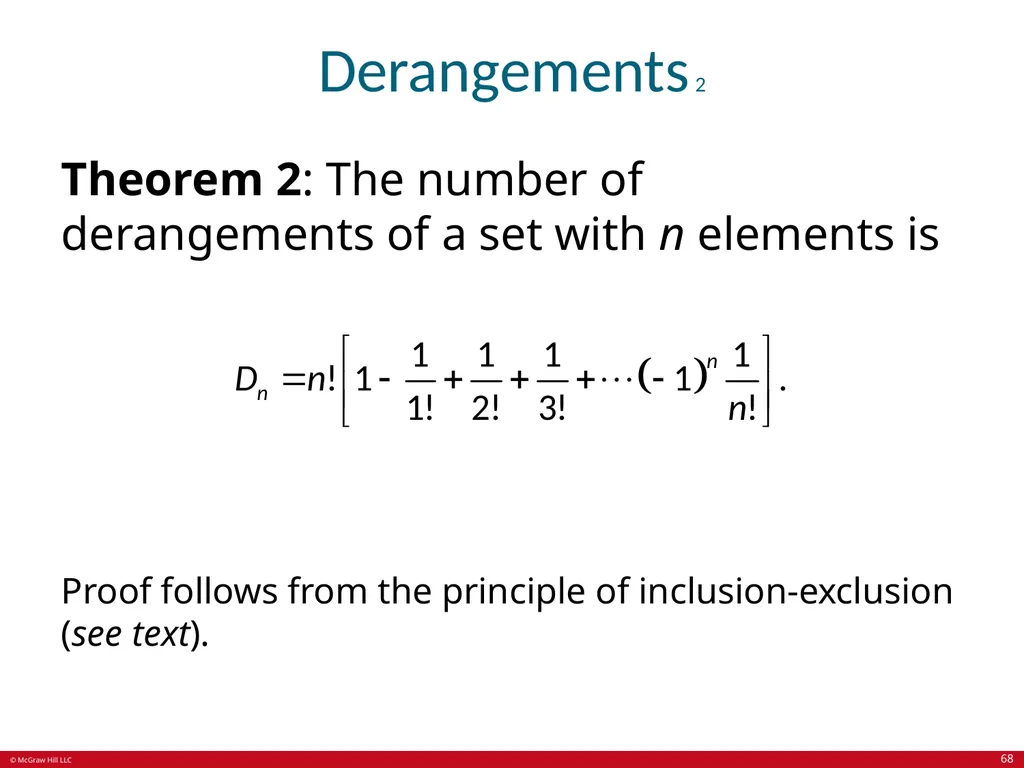
slide68. Derangements 2 Theorem 2: The number of derangements of a set with n elements is Proof follows from the principle of inclusion-exclusion (see text). 68<br>
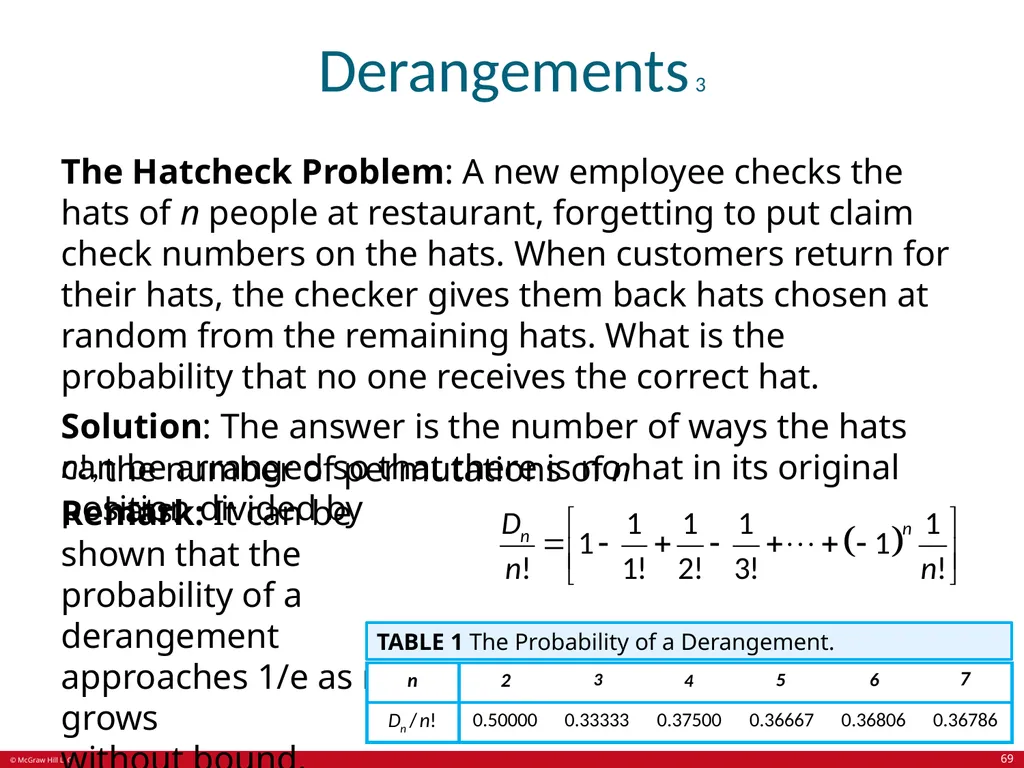
slide69. Derangements 3 The Hatcheck Problem: A new employee checks the hats of n people at restaurant, forgetting to put claim check numbers on the hats. When customers return for their hats, the checker gives them back hats chosen at random from the remaining hats. What is the probability that no one receives the correct hat.
Solution: The answer is the number of ways the hats can be arranged so that there is no hat in its original position divided by the number of permutations of n hats. Remark: It can be shown that the probability of a derangement approaches 1/e as n growswithout bound. TABLE 1 The Probability of a Derangement. 69<br>
slide70. End of Main Content © McGraw Hill LLC. All rights reserved. No reproduction or distribution without the prior written consent of McGraw Hill LLC.<br>
slide71. Accessibility Content: Text Alternatives for Images 71<br>
slide72. Rabbits and the Fibonacci Numbers 2 – Text Alternative Return to parent-slide containing images. There is 0 reproducing pair and 1 young pair in the first month, the number of total pairs is 1. There is 0 reproducing pair and 1 young pair in the second month, the number of total pairs is 1. There is 1 reproducing pair and 1 young pair in the third month, the number of total pairs is 2. There is 1 reproducing pair and 2 young pairs in the fourth month, the number of total pairs is 3. There are 2 reproducing pairs and 3 young pairs in the fifth month, the number of total pairs is 5. There are 3 reproducing pairs and 5 young pairs in the sixth month, the number of total pairs is 8. Return to parent-slide containing images. 72<br>
slide73. Counting Bit Strings 1 – Text Alternative Return to parent-slide containing images. The first bit string starts with any bit string of length N minus 1 with no two consecutive zeros and ends with a 1. The number of strings of this type is A sub, N minus 1. The second bit strings starts with any bit string of length N minus 2 with no two consecutive zeros and ends with 1 0. The number of strings of this type is A sub, N minus 2. The total number of bit strings of length N with no two consecutive zeros is A sub, N minus 1, plus A sub, N minus 2. Return to parent-slide containing images. 73<br>
slide74. Useful Generating Functions – Text Alternative Return to parent-slide containing images. The column headers are marked as: G(x) and ak.The data is as follows:Row 1: (1 plus x) to the power n equals summation from k equals 0 through n C (n, k) times x to the power k equals 1 plus c (n, 1)x plus C (n, 2) x squared plus .. plus x to the power n and C (n, k).Row 2: (1 plus a times x) to the power n equals summation from k equals 0 through n C (n, k) a to the power k x to the power k equals 1 plus C (n, 1) a times x plus C (n, 2) a squared times x squared plus .. plus a to the power n times x to the power n and C (n, k) times a to the power k.Row 3: (1 plus x to the power r) to the power n equals summation from k equals 0 through n C (n, k) times x to the power r times k equals 1 plus C (n, 1) x to the power r plus C (n, 2) times x to the power 2 times r plus .. plus x to the power r times n and C (n, k over r) if r|k; 0 otherwise.Row 4: Fraction 1 minus x to the power n plus 1 over 1 minus x equals summation from k equals 0 through infinity x to the power k equals 1 plus x plus x squared plus... x to the power n and 1 if k lesser than or equal to n; 0 otherwise.Row 5: Fraction 1 over 1 minus x equals summation from k equals 0 through infinity x to the power k equals 1 plus x plus x squared plus ... and 1.Row 6: Fraction 1 over 1 minus a times x equals summation from k equals 0 through infinity a to the power k times x to the power k equals 1 plus a times x plus a squared times x squared plus .. and a to the power k.Row 7: 1 over 1 minus x to the power r equals summation from k equals 0 through infinity equals 1 plus x to the power r plus x to the power 2 times r and 1 if r|k; otherwise.Row 8: Fraction 1 over (1 minus x) squared equals summation 0 through infinity (k plus 1) x to the power k equals 1 plus 2 times x plus 3 times x squared, and k plus 1. Row 9: Fraction 1 over (1 minus x) to the power n equals summation from k equals 0 through infinity C (n plus k minus 1, k) times x to the power k equals 1 plus C (n, 1) times x plus c (n plus 1, 2) times x squared plus .. and C (n plus k minus 1, k) equals C (n plus k minus 1, n minus 1).Row 10: Fraction 1 over (1 plus x) to the power n equals summation k equals 0 through infinity C (n plus k minus 1, k) times (negative 1) to the power k times x to the power k equals 1 minus C (n, 1) times x plus C (n plus 1, 2) x squared.. and (negative 1) to the power k times C (n plus k minus 1, k) equals (negative 1) to the power k times C (n plus k minus 1, n minus 1).Row 11: Fraction 1 over (1 minus a times x) to the power n equals summation k equals 0 through infinity C (n plus k minus 1, k) times a to the power k times x to the power k equals 1 plus C (n, 1) times a times x plus C (n plus 1, 2) times a squared times x squared plus .. and C (n plus k minus 1, k) times a to the power k) equals C (n plus k minus 1, n minus 1) times a to the power k.Row 12: e to the power x equals summation k equals 0 through infinity fraction x to the power k over k factorial equals 1 plus x plus fraction x squared over 2 factorial plus fraction x cubed over 3 factorial plus .. and 1 over k factorial.Row 13: ln (1 plus x) equals summation k equals 1 through infinity fraction (negative 1) to the power k plus 1 over k times x to the power k equals x minus fraction x squared over 2 plus fraction x cubed over 3 minus x to the power 4 over 4 plus .. and (negative 1) to the power k plus 1 over k. Return to parent-slide containing images. 74<br>
slide75. Two Finite Sets – Text Alternative Return to parent-slide containing images. The number of elements in A is 25, the number of elements in B is 13. The number of elements in the intersection of A and B is 8. Return to parent-slide containing images. 75<br>
slide76. Three Finite Sets 1 – Text Alternative Return to parent-slide containing images. The first diagram shows count of elements by the formula number of elements in A plus the number of elements in B plus the number of elements in C. There is number 1 in exactly one of the three sets, number 2 in the intersection of any two of the sets, and number 3 in the intersection of all three sets. The second diagram shows count of elements by the formula number of elements in A plus the number of elements in B plus the number of elements in C minus the number of elements in intersection of A and B minus the number of elements in intersection of A and C minus the number of elements in intersection of B and C. There is number 1 in exactly one of the three sets and in the intersection of any two of the sets, and number 0 in the intersection of all three sets. The third diagram shows count of elements by the formula number of elements in A plus the number of elements in B plus the number of elements in C minus the number of elements in intersection of A and B minus the number of elements in intersection of A and C minus the number of elements in intersection of B and C plus the number of elements in intersection of A, B, and C. There is number 1 in exactly one of the three sets and in all intersections. Return to parent-slide containing images. 76<br>
slide77. Illustration of Three Finite Set Example – Text Alternative Return to parent-slide containing images. The number of elements for the sets are given below: Set S = 1232Set F = 879Set R = 114Intersection of sets S and R = 23Intersection of sets F and R = 14Intersection of sets S and F = 103Union of sets S, F, and R = 2092 Return to parent-slide containing images. 77<br>