04
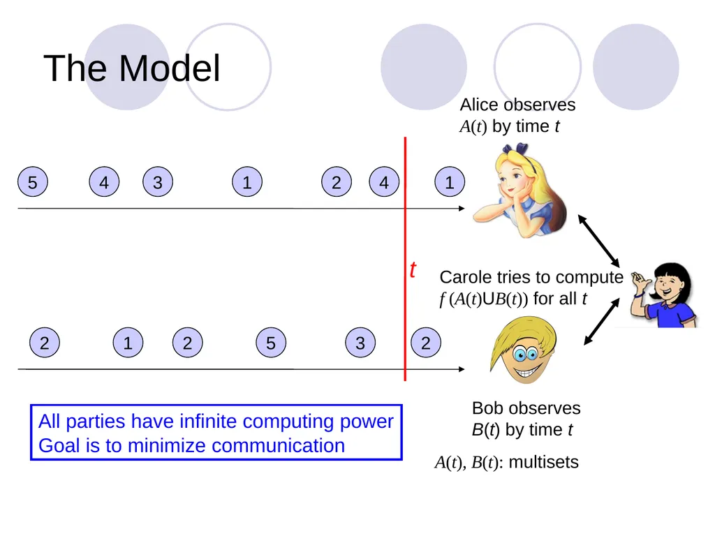
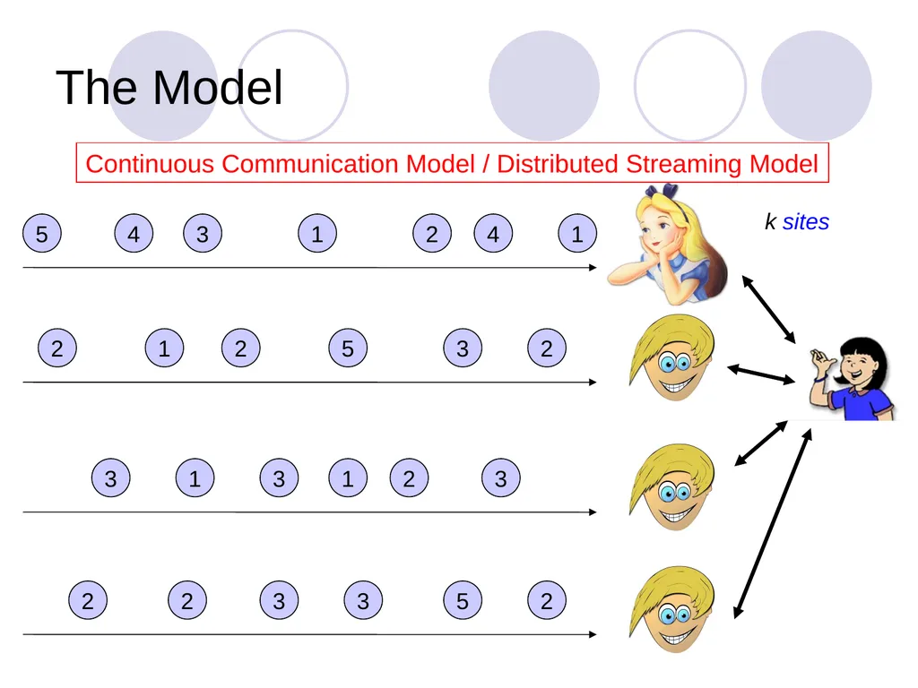
The Model 1 4 2 1 3 4 5 2 3 5 2 1 2 2 3 1 3 1 3 2 5 3 3 2 2 k sites Continuous Communication Model / Distributed Streaming Model<br>
05
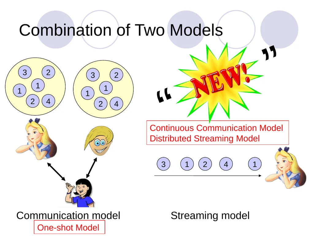
Combination of Two Models 3 1 1 2 4 2 3 1 1 2 4 2 Communication model 1 4 2 1 3 Streaming model Continuous Communication Model �Distributed Streaming Model One-shot Model “ ”<br>
06
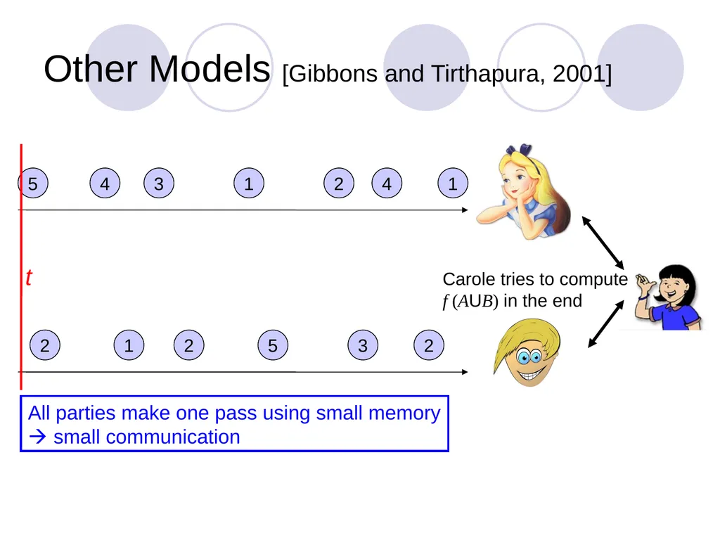
Other Models [Gibbons and Tirthapura, 2001] 1 4 2 1 3 4 5 2 3 5 2 1 2 Carole tries to compute�f (AUB) in the end All parties make one pass using small memory
small communication t<br>
07
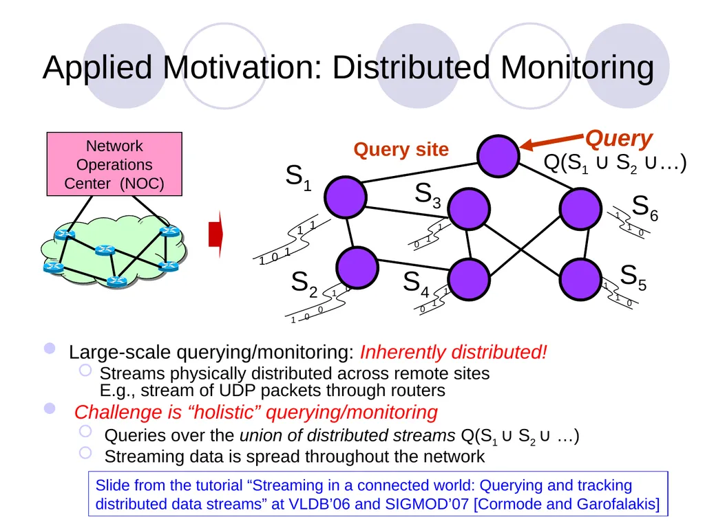
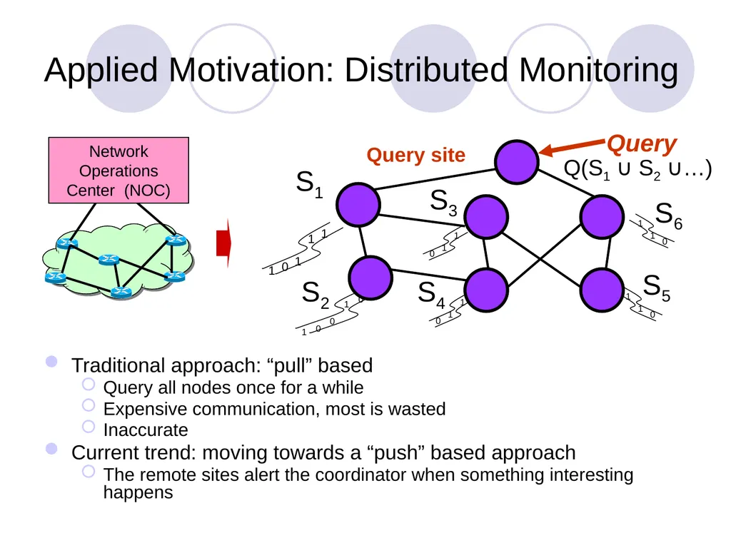
Applied Motivation: Distributed Monitoring Large-scale querying/monitoring: Inherently distributed!
Streams physically distributed across remote sites�E.g., stream of UDP packets through routers
Challenge is “holistic” querying/monitoring
Queries over the union of distributed streams Q(S1 ∪ S2 ∪ …)
Streaming data is spread throughout the network Network Operations
Center (NOC) Slide from the tutorial “Streaming in a connected world: Querying and tracking�distributed data streams” at VLDB’06 and SIGMOD’07 [Cormode and Garofalakis]<br>
08
Applied Motivation: Distributed Monitoring Traditional approach: “pull” based
Query all nodes once for a while
Expensive communication, most is wasted
Inaccurate
Current trend: moving towards a “push” based approach
The remote sites alert the coordinator when something interesting happens Network Operations
Center (NOC)<br>
09
Theoretical Questions Upper bounds: Worst-case communication bounds for a given f ?
Lower bounds: Is there a gap in the communication complexity between the one-shot model and the continuous model?<br>
10
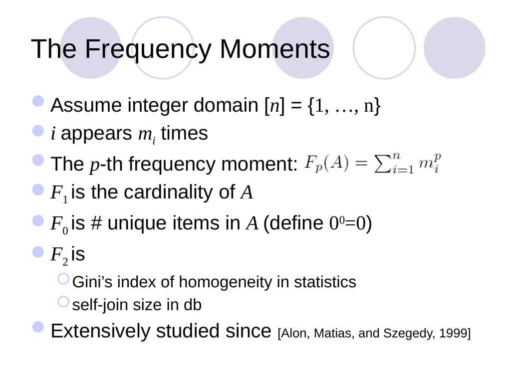
The Frequency Moments Assume integer domain [n] = {1, …, n}
i appears mi times
The p-th frequency moment:
F1 is the cardinality of A
F0 is # unique items in A (define 00=0)
F2 is
Gini’s index of homogeneity in statistics
self-join size in db
Extensively studied since [Alon, Matias, and Szegedy, 1999]<br>
11
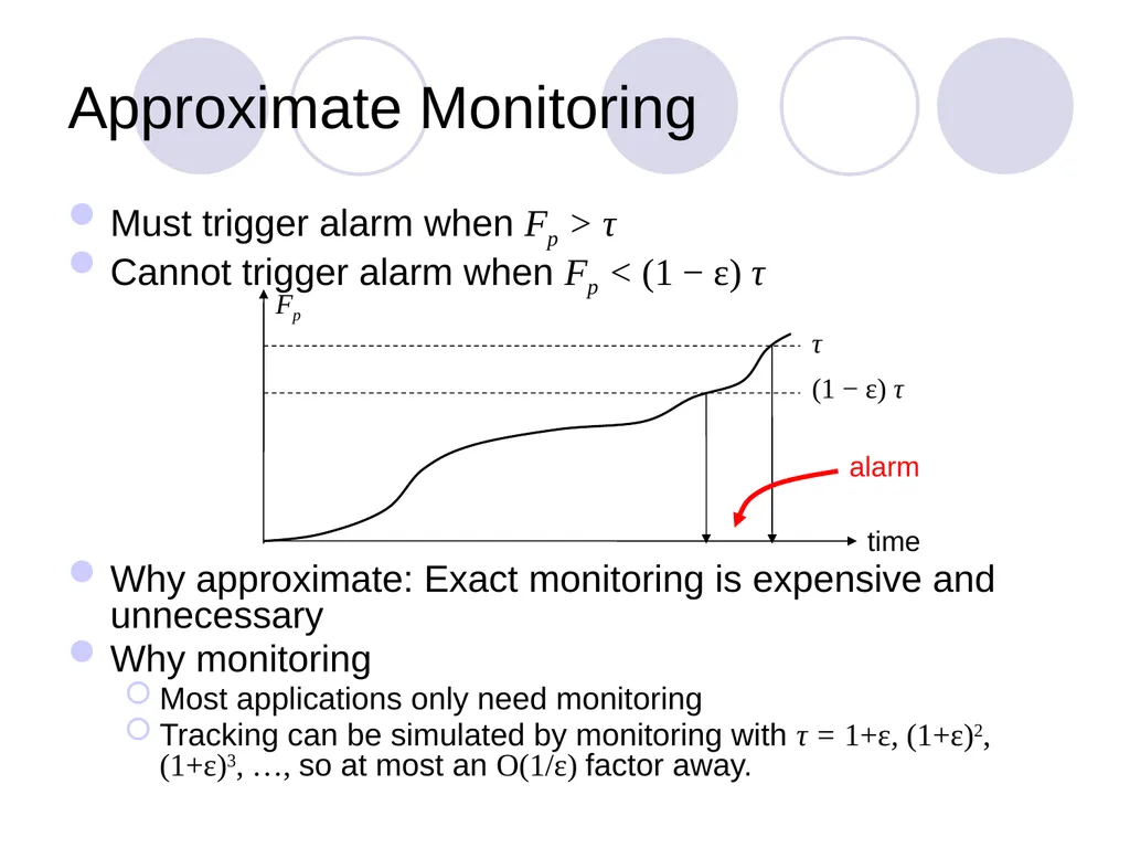
Approximate Monitoring Must trigger alarm when Fp > τ
Cannot trigger alarm when Fp < (1 − ε) τ
Why approximate: Exact monitoring is expensive and unnecessary
Why monitoring
Most applications only need monitoring
Tracking can be simulated by monitoring with τ = 1+ε, (1+ε)2, (1+ε)3, …, so at most an O(1/ε) factor away. time Fp τ (1 − ε) τ alarm<br>
12
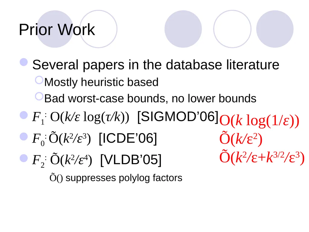
Prior Work Several papers in the database literature
Mostly heuristic based
Bad worst-case bounds, no lower bounds
F1: O(k/ε log(τ/k)) [SIGMOD’06]
F0: Õ(k2/ε3) [ICDE’06]
F2: Õ(k2/ε4) [VLDB’05]
Õ() suppresses polylog factors O(k log(1/ε))
Õ(k/ε2)
Õ(k2/ε+k3/2/ε3)<br>
13
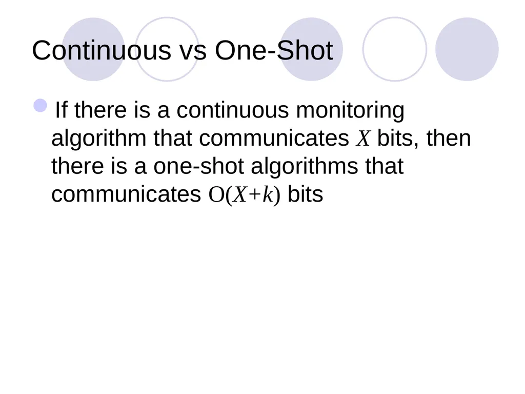
Continuous vs One-Shot If there is a continuous monitoring algorithm that communicates X bits, then there is a one-shot algorithms that communicates O(X+k) bits<br>
14
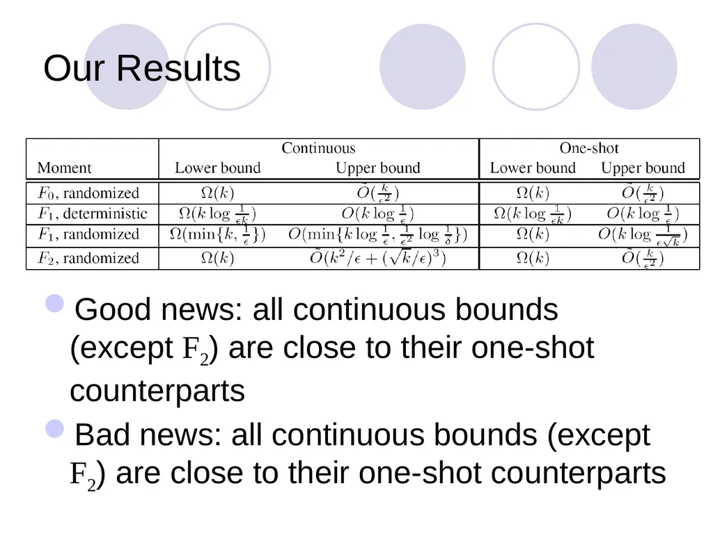
Our Results Good news: all continuous bounds (except F2) are close to their one-shot counterparts
Bad news: all continuous bounds (except F2) are close to their one-shot counterparts<br>
15
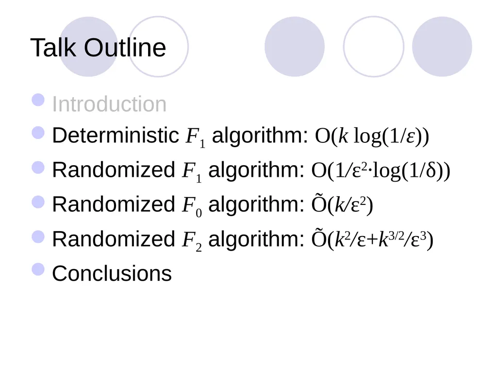
Talk Outline Introduction
Deterministic F1 algorithm: O(k log(1/ε))
Randomized F1 algorithm: O(1/ε2∙log(1/δ))
Randomized F0 algorithm: Õ(k/ε2)
Randomized F2 algorithm: Õ(k2/ε+k3/2/ε3)
Conclusions<br>
16
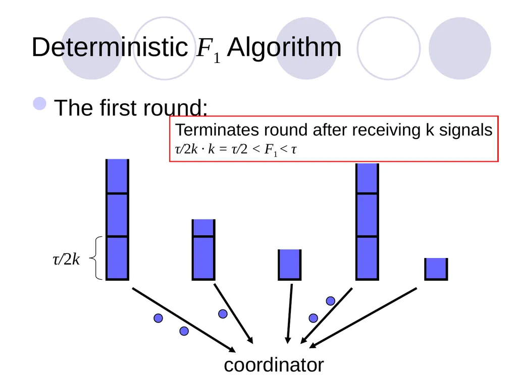
Deterministic F1 Algorithm The first round: τ/2k coordinator Terminates round after receiving k signals
τ/2k · k = τ/2 < F1 < τ<br>
17
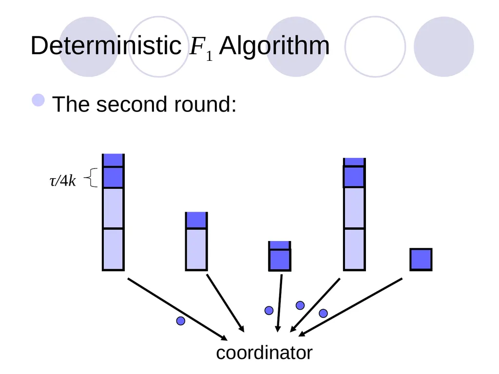
Deterministic F1 Algorithm The second round: τ/4k coordinator<br>
18
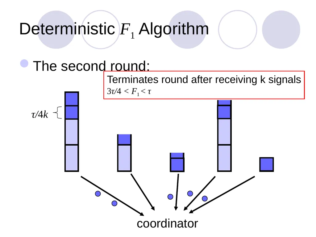
Deterministic F1 Algorithm The second round: τ/4k coordinator Terminates round after receiving k signals
3τ/4 < F1 < τ<br>
19
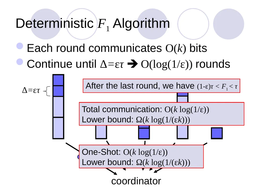
Deterministic F1 Algorithm Each round communicates O(k) bits
Continue until Δ=ετ O(log(1/ε)) rounds Δ=ετ coordinator After the last round, we have (1-ε)τ < F1 < τ Total communication: O(k log(1/ε))
Lower bound: Ω(k log(1/(εk))) One-Shot: O(k log(1/ε))
Lower bound: Ω(k log(1/(εk)))<br>
20
Talk Outline Introduction
Deterministic F1 algorithm: O(k log(1/ε))
Randomized F1 algorithm: O(1/ε2∙log(1/δ))
Randomized F0 algorithm: Õ(k/ε2)
Randomized F2 algorithm: Õ(k2/ε+k3/2/ε3)
Conclusions<br>
21
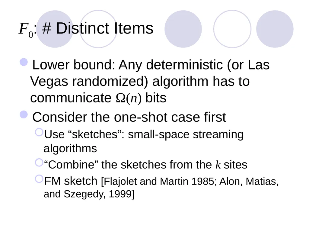
F0: # Distinct Items Lower bound: Any deterministic (or Las Vegas randomized) algorithm has to communicate Ω(n) bits
Consider the one-shot case first
Use “sketches”: small-space streaming algorithms
“Combine” the sketches from the k sites
FM sketch [Flajolet and Martin 1985; Alon, Matias, and Szegedy, 1999]<br>
22
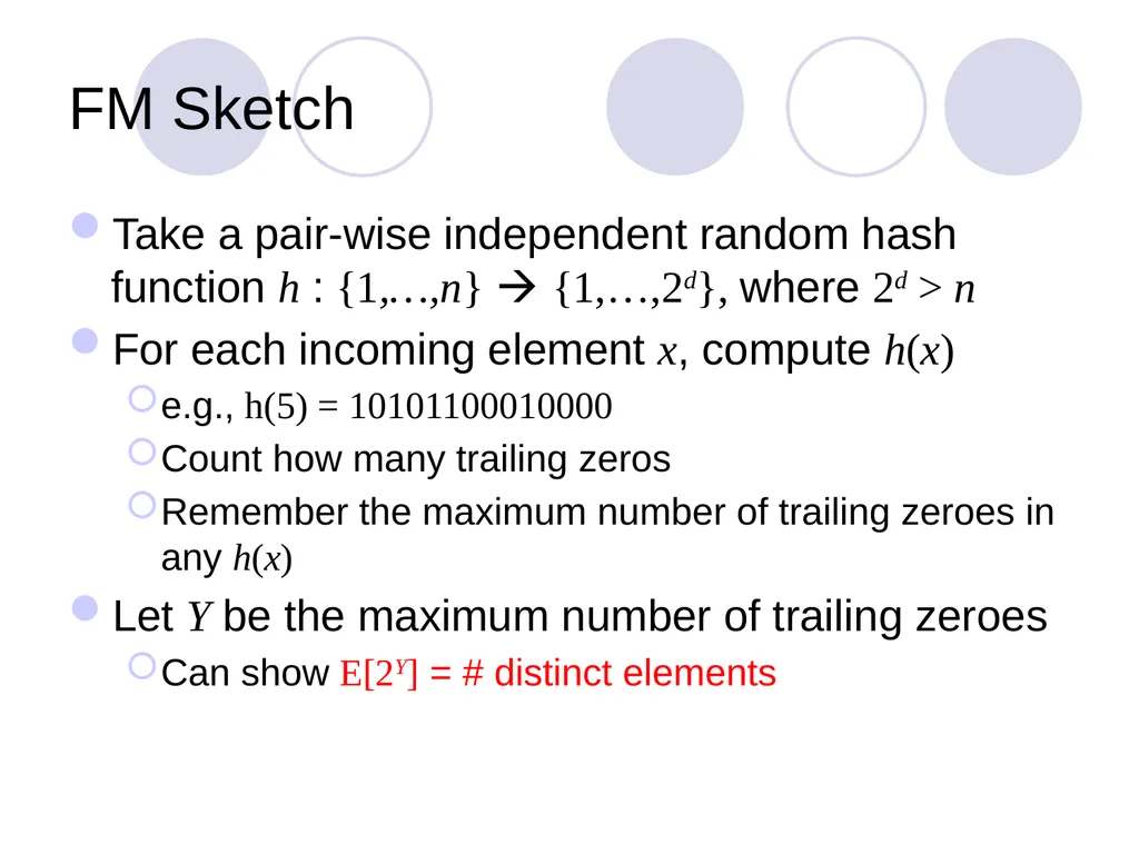
FM Sketch Take a pair-wise independent random hash function h : {1,…,n} {1,…,2d}, where 2d > n
For each incoming element x, compute h(x)
e.g., h(5) = 10101100010000
Count how many trailing zeros
Remember the maximum number of trailing zeroes in any h(x)
Let Y be the maximum number of trailing zeroes
Can show E[2Y] = # distinct elements<br>
23
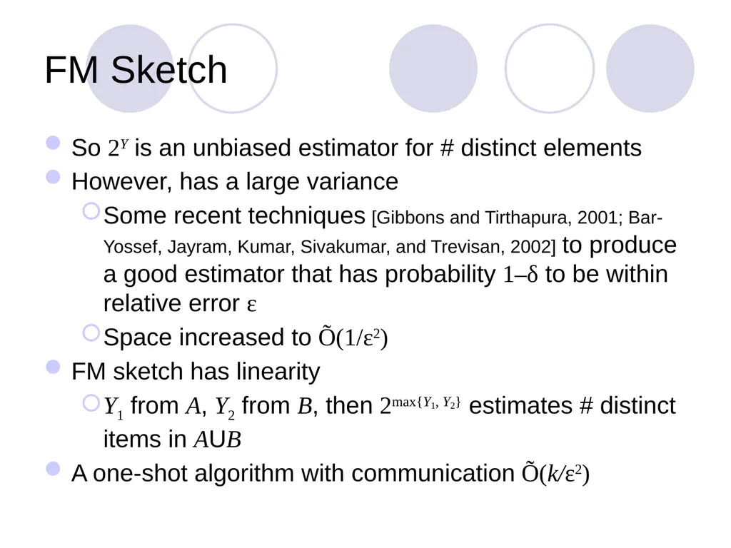
FM Sketch So 2Y is an unbiased estimator for # distinct elements
However, has a large variance
Some recent techniques [Gibbons and Tirthapura, 2001; Bar-Yossef, Jayram, Kumar, Sivakumar, and Trevisan, 2002] to produce a good estimator that has probability 1–δ to be within relative error ε
Space increased to Õ(1/ε2)
FM sketch has linearity
Y1 from A, Y2 from B, then 2max{Y1, Y2} estimates # distinct items in AUB
A one-shot algorithm with communication Õ(k/ε2)<br>
24
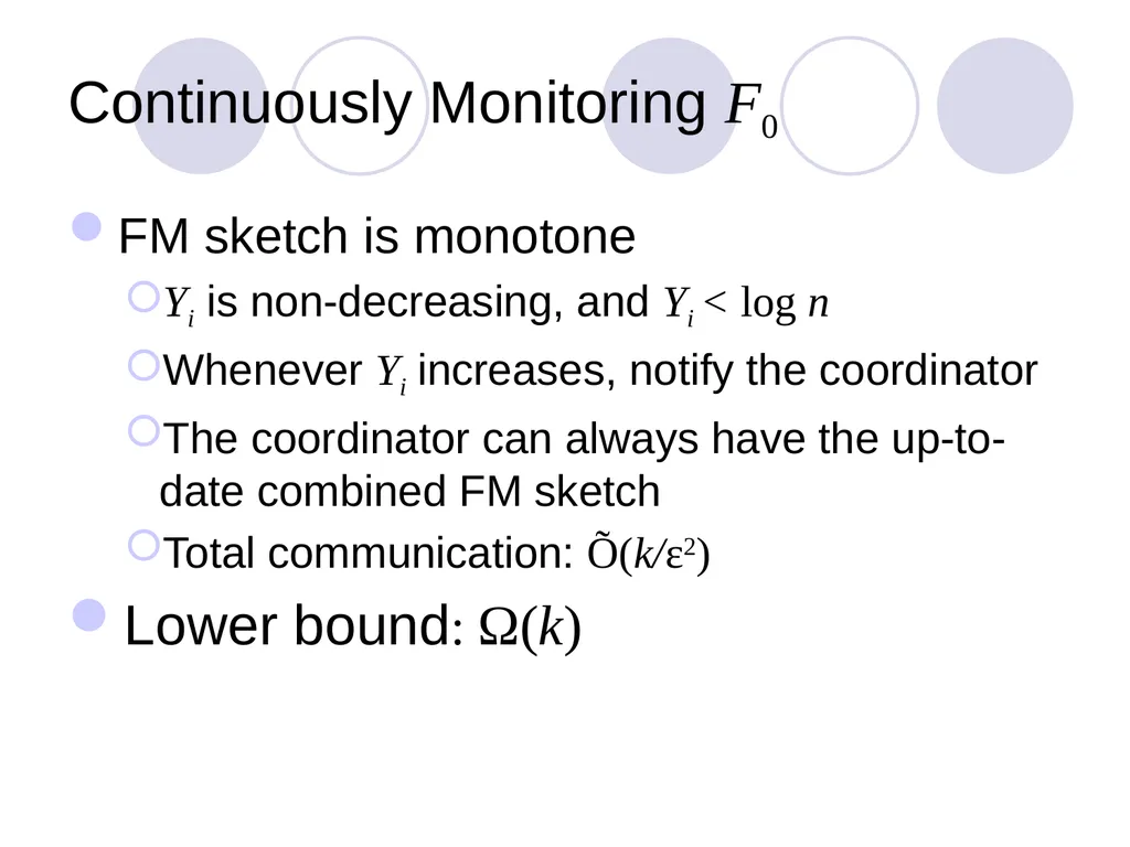
Continuously Monitoring F0 FM sketch is monotone
Yi is non-decreasing, and Yi < log n
Whenever Yi increases, notify the coordinator
The coordinator can always have the up-to-date combined FM sketch
Total communication: Õ(k/ε2)
Lower bound: Ω(k)<br>
25
Talk Outline Introduction
Deterministic F1 algorithm: O(k log(1/ε))
Randomized F1 algorithm: O(1/ε2∙log(1/δ))
Randomized F0 algorithm: Õ(k/ε2)
Randomized F2 algorithm: Õ(k2/ε+k3/2/ε3)
Conclusions<br>
26
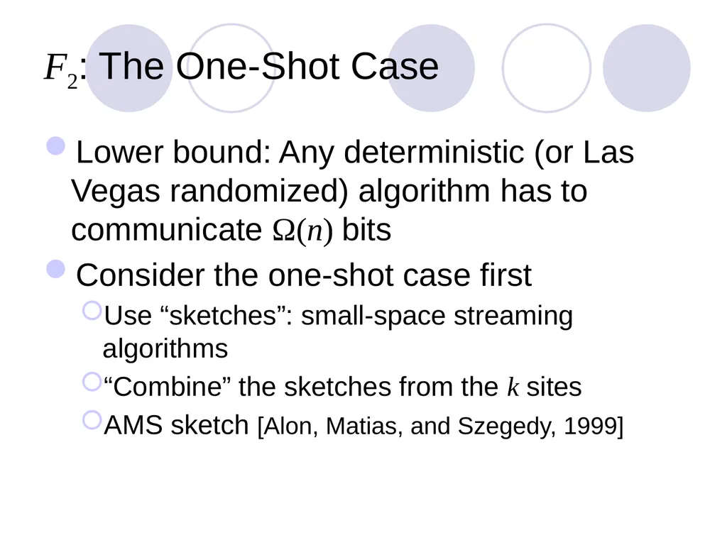
F2: The One-Shot Case Lower bound: Any deterministic (or Las Vegas randomized) algorithm has to communicate Ω(n) bits
Consider the one-shot case first
Use “sketches”: small-space streaming algorithms
“Combine” the sketches from the k sites
AMS sketch [Alon, Matias, and Szegedy, 1999]<br>
27
AMS Sketch: “Tug-of-War” Take a 4-wise independent random hash function�h : {1,…,n} {−1,+1}
Compute
Y = ∑ h(x)
over all x
Y2 is an unbiased estimator for F2
Use O(1/ε2 ∙ log(1/δ)) copies to guarantee a good estimator that has probability 1–δ to be within relative error ε
Linearity still holds!
One-shot case can be solved with communication Õ(k/ε2)<br>
28
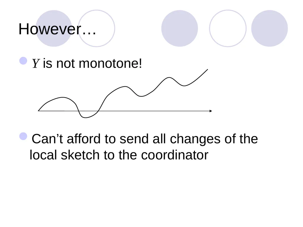
However… Y is not monotone!
Can’t afford to send all changes of the local sketch to the coordinator<br>
29
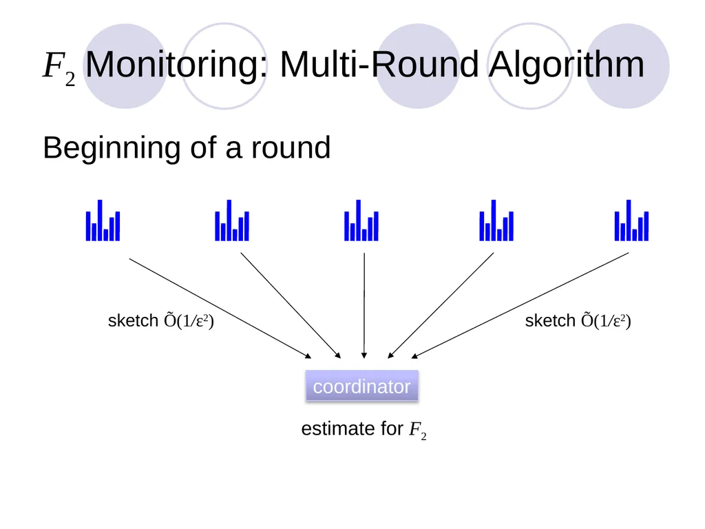
F2 Monitoring: Multi-Round Algorithm Beginning of a round sketch Õ(1/ε2) sketch Õ(1/ε2) estimate for F2 coordinator<br>
30
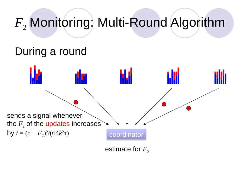
F2 Monitoring: Multi-Round Algorithm During a round estimate for F2 coordinator sends a signal whenever�the F2 of the updates increases�by t = (τ − F2)2/(64k2τ)<br>
31
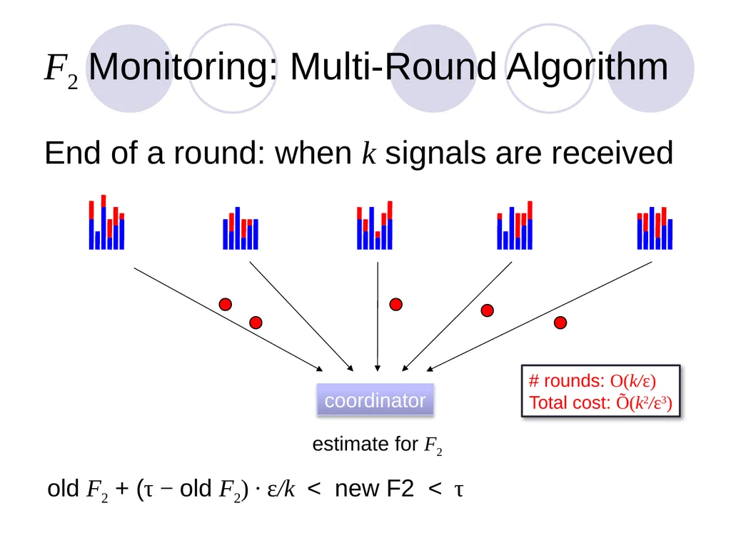
F2 Monitoring: Multi-Round Algorithm End of a round: when k signals are received estimate for F2 coordinator old F2 + (τ − old F2) ∙ ε/k < new F2 < τ # rounds: O(k/ε)
Total cost: Õ(k2/ε3)<br>
32
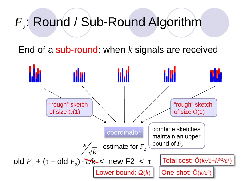
F2: Round / Sub-Round Algorithm End of a sub-round: when k signals are received estimate for F2 coordinator old F2 + (τ − old F2) ∙ ε/k < new F2 < τ “rough” sketch
of size Õ(1) “rough” sketch
of size Õ(1) combine sketches
maintain an upper bound of F2 Total cost: Õ(k2/ε+k3/2/ε3) One-shot: Õ(k/ε2) Lower bound: Ω(k)<br>
33
Open Problems Still no clear separation between the one-shot model and the continuous model
F2 is an interesting case
Many other functions f
Statistics: entropy, heavy hitters
Geometric measures: diameter, width, …
Variations of the model
One-way vs two-way communication
Does having a broadcast channel help?
Sliding windows?
“Continuous Communication Complexity”?<br>