Artificial Neural Networks 1 2 Neural networks

slide1. Artificial Neural Networks 1<br>
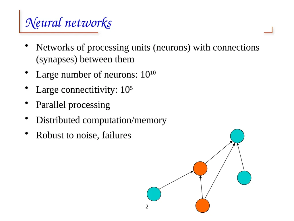
slide2. 2 Neural networks Networks of processing units (neurons) with connections (synapses) between them
Large number of neurons: 1010
Large connectitivity: 105
Parallel processing
Distributed computation/memory
Robust to noise, failures<br>
slide3. Connectionism Alternative to symbolism
Humans and evidence of connectionism/parallelism:
Physical structure of brain:
Neuron switching time: 10-3 second
Complex, short-time computations:
Scene recognition time: 10-1 second
100 inference steps doesn’t seem like enough
much parallel computation
Artificial Neural Networks (ANNs)
Many neuron-like threshold switching units
Many weighted interconnections among units
Highly parallel, distributed process
Emphasis on tuning weights automatically (search in weight space) 3<br>
slide4. Biological neuron video<br>
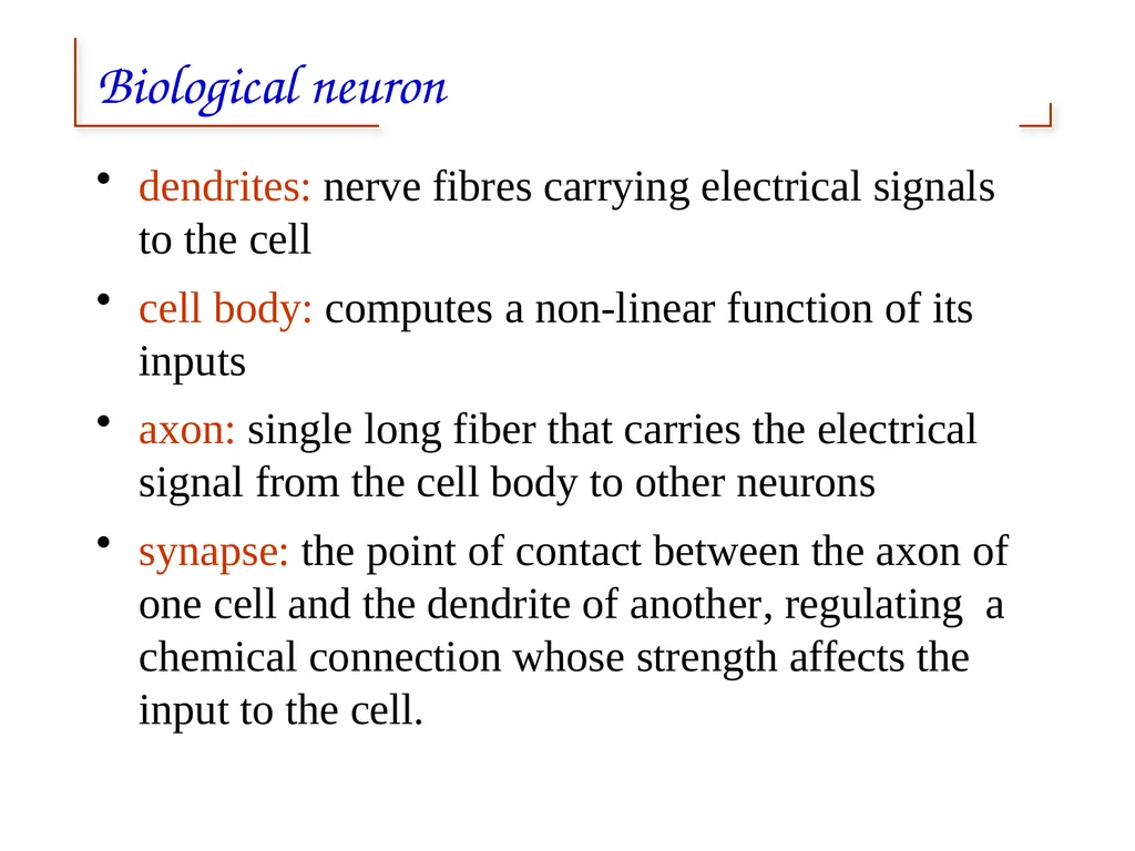
slide5. Biological neuron dendrites: nerve fibres carrying electrical signals to the cell
cell body: computes a non-linear function of its inputs
axon: single long fiber that carries the electrical signal from the cell body to other neurons
synapse: the point of contact between the axon of one cell and the dendrite of another, regulating a chemical connection whose strength affects the input to the cell.<br>
slide6. Biological neuron A variety of different neurons exist (motor neuron, on-center off-surround visual cells…), with different branching structures
The connections of the network and the strengths of the individual synapses establish the function of the network.<br>
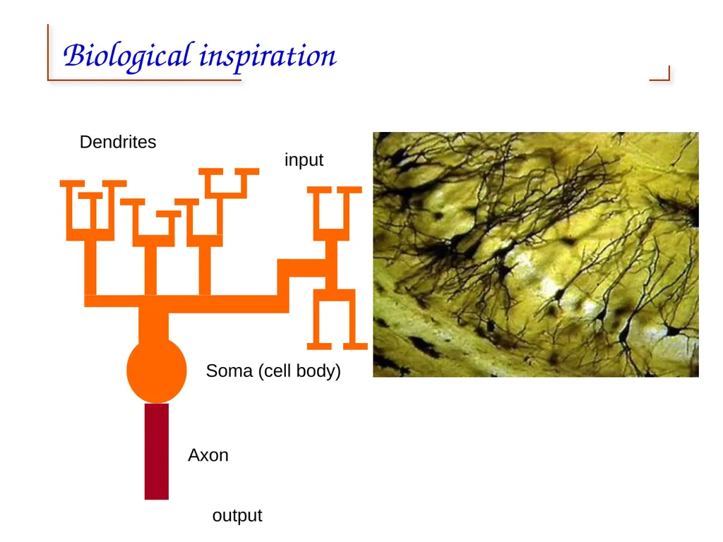
slide7. Biological inspiration Dendrites Soma (cell body) Axon input output<br>
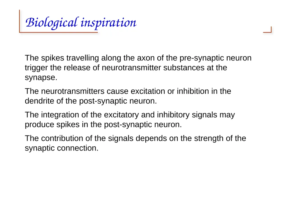
slide8. Biological inspiration The spikes travelling along the axon of the pre-synaptic neuron trigger the release of neurotransmitter substances at the synapse.
The neurotransmitters cause excitation or inhibition in the dendrite of the post-synaptic neuron.
The integration of the excitatory and inhibitory signals may produce spikes in the post-synaptic neuron.
The contribution of the signals depends on the strength of the synaptic connection.<br>
slide9. Hodgkin and Huxley model Hodgkin and Huxley experimented on squids and discovered how the signal is produced within the neuron
This model was published in Jour. of Physiology (1952)
They were awarded the 1963 Nobel Prize<br>
slide10. When to consider ANNs Input is
high-dimensional
discrete or real-valued
e.g., raw sensor inputs
noisy
Long training times
Form of target function is unknown
Human readability is unimportant
Especially good for complex recognition problems
Speech recognition
Image classification
Financial prediction 10<br>
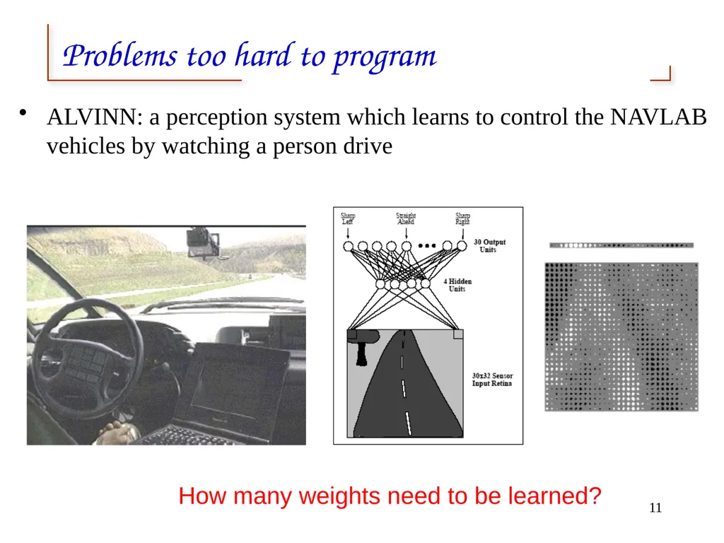
slide11. Problems too hard to program ALVINN: a perception system which learns to control the NAVLAB vehicles by watching a person drive 11 How many weights need to be learned?<br>
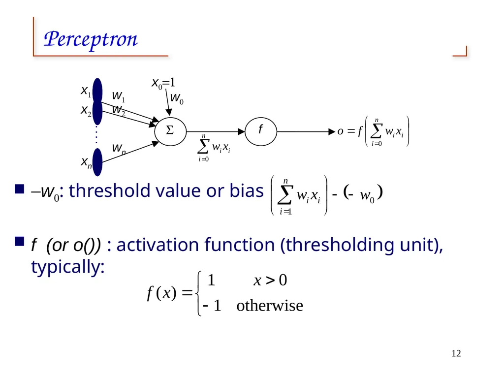
slide12. Perceptron -w0: threshold value or bias

f (or o()) : activation function (thresholding unit), typically: x1 x2 xn w1 w2 wn :: x0=1 w0 S f 12<br>
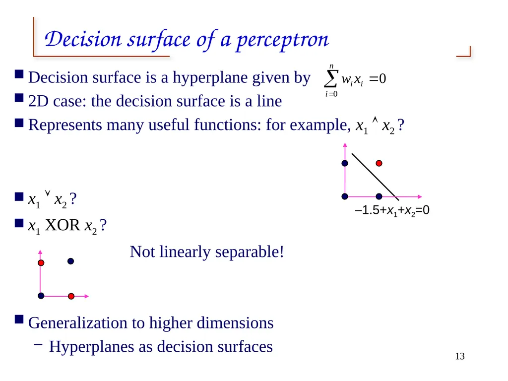
slide13. Decision surface of a perceptron Decision surface is a hyperplane given by
2D case: the decision surface is a line
Represents many useful functions: for example, x1  x2 ?

x1  x2 ?
x1 XOR x2 ?
Not linearly separable!

Generalization to higher dimensions
Hyperplanes as decision surfaces 13<br>
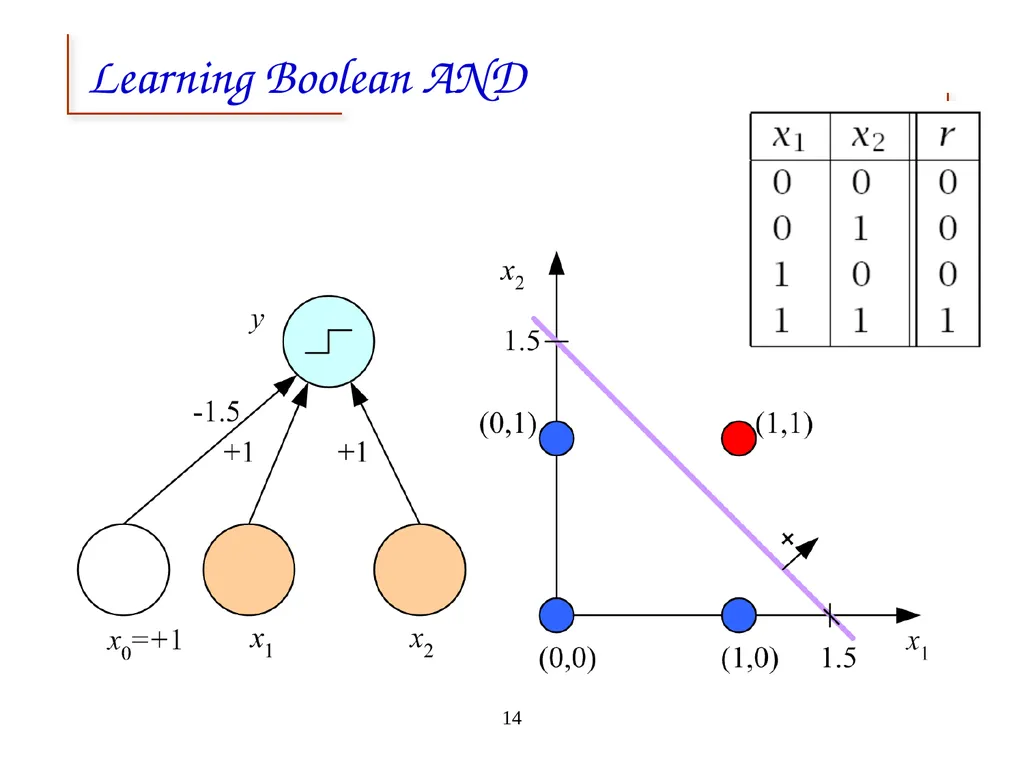
slide14. 14 Learning Boolean AND<br>
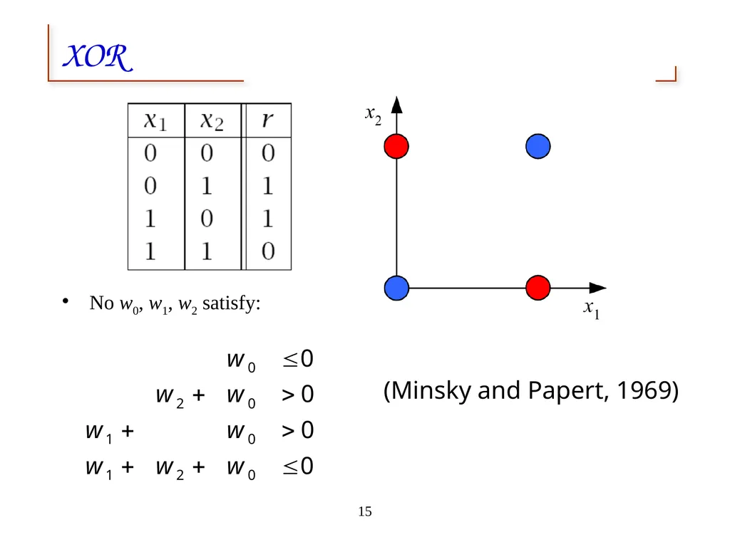
slide15. 15 XOR No w0, w1, w2 satisfy: (Minsky and Papert, 1969)<br>
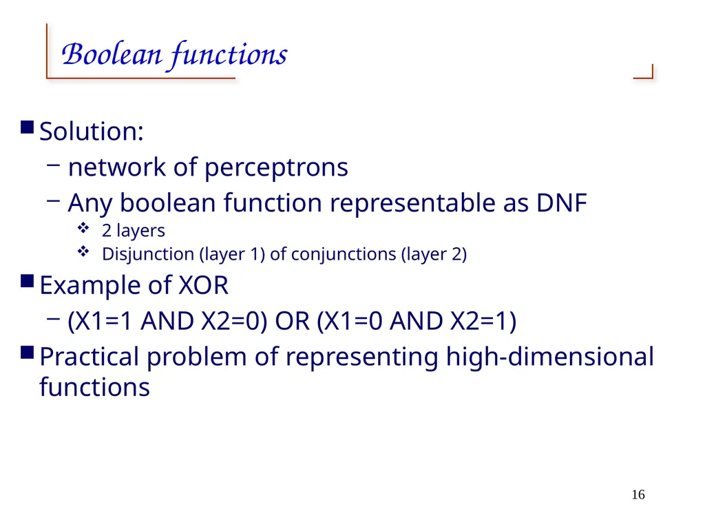
slide16. Boolean functions Solution:
network of perceptrons
Any boolean function representable as DNF
2 layers
Disjunction (layer 1) of conjunctions (layer 2)
Example of XOR
(X1=1 AND X2=0) OR (X1=0 AND X2=1)
Practical problem of representing high-dimensional functions 16<br>
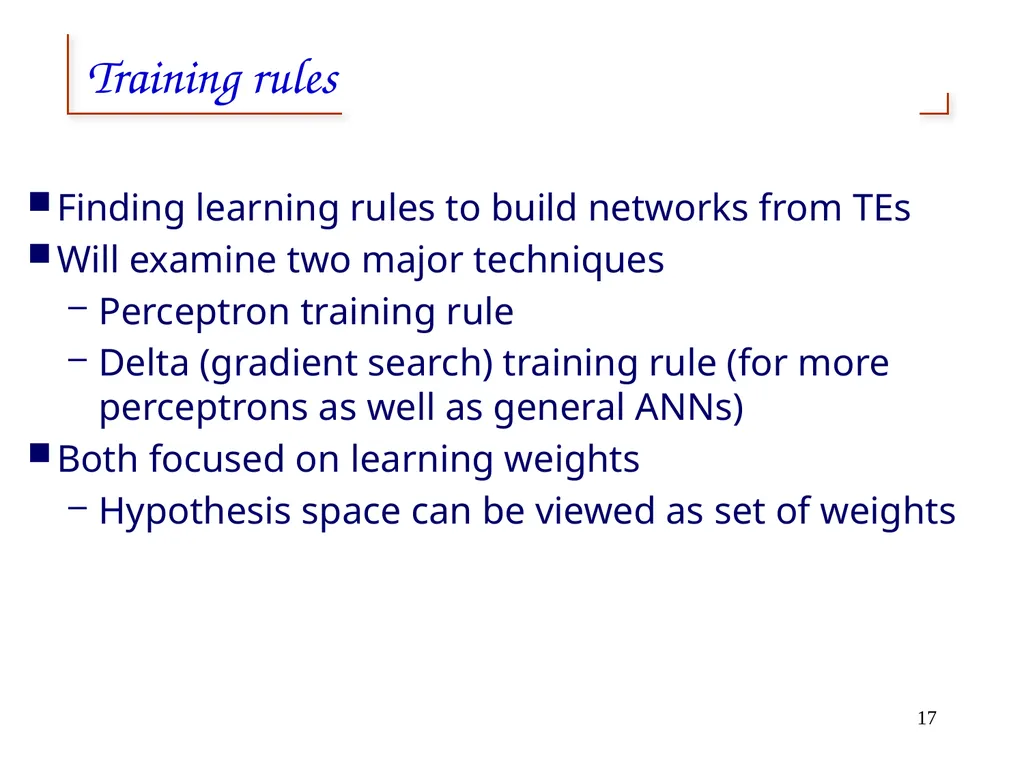
slide17. Training rules Finding learning rules to build networks from TEs
Will examine two major techniques
Perceptron training rule
Delta (gradient search) training rule (for more perceptrons as well as general ANNs)
Both focused on learning weights
Hypothesis space can be viewed as set of weights 17<br>
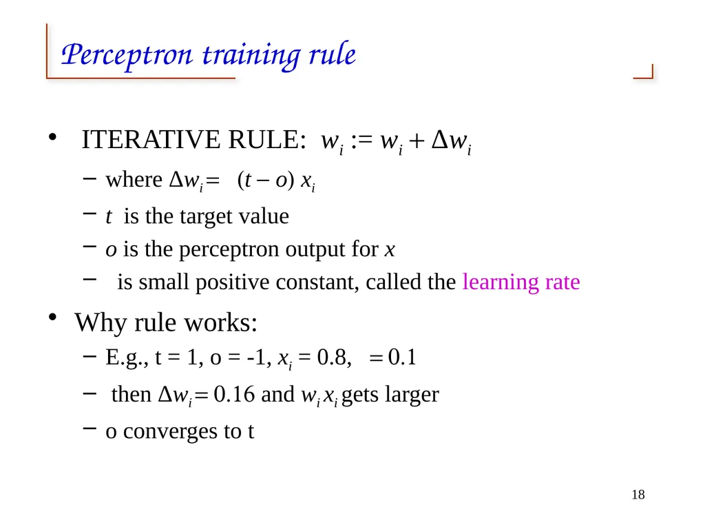
slide18. Perceptron training rule ITERATIVE RULE: wi := wi + Δwi
where Δwi =  (t - o) xi
t is the target value
o is the perceptron output for x
 is small positive constant, called the learning rate
Why rule works:
E.g., t = 1, o = -1, xi = 0.8,  = 0.1
then Δwi = 0.16 and wi xi gets larger
o converges to t 18<br>
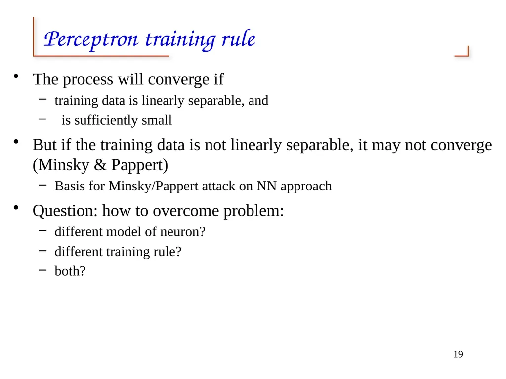
slide19. Perceptron training rule The process will converge if
training data is linearly separable, and
 is sufficiently small
But if the training data is not linearly separable, it may not converge (Minsky & Pappert)
Basis for Minsky/Pappert attack on NN approach
Question: how to overcome problem:
different model of neuron?
different training rule?
both? 19<br>
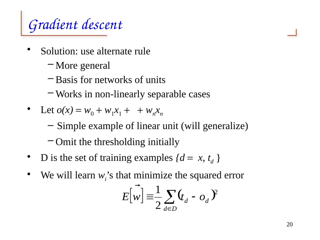
slide20. Gradient descent Solution: use alternate rule
More general
Basis for networks of units
Works in non-linearly separable cases
Let o(x) = w0 + w1x1 +  + wnxn
Simple example of linear unit (will generalize)
Omit the thresholding initially
D is the set of training examples {d = x, td}
We will learn wi’s that minimize the squared error 20<br>
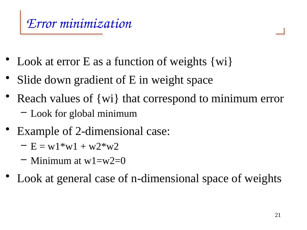
slide21. Error minimization Look at error E as a function of weights {wi}
Slide down gradient of E in weight space
Reach values of {wi} that correspond to minimum error
Look for global minimum
Example of 2-dimensional case:
E = w1*w1 + w2*w2
Minimum at w1=w2=0
Look at general case of n-dimensional space of weights 21<br>
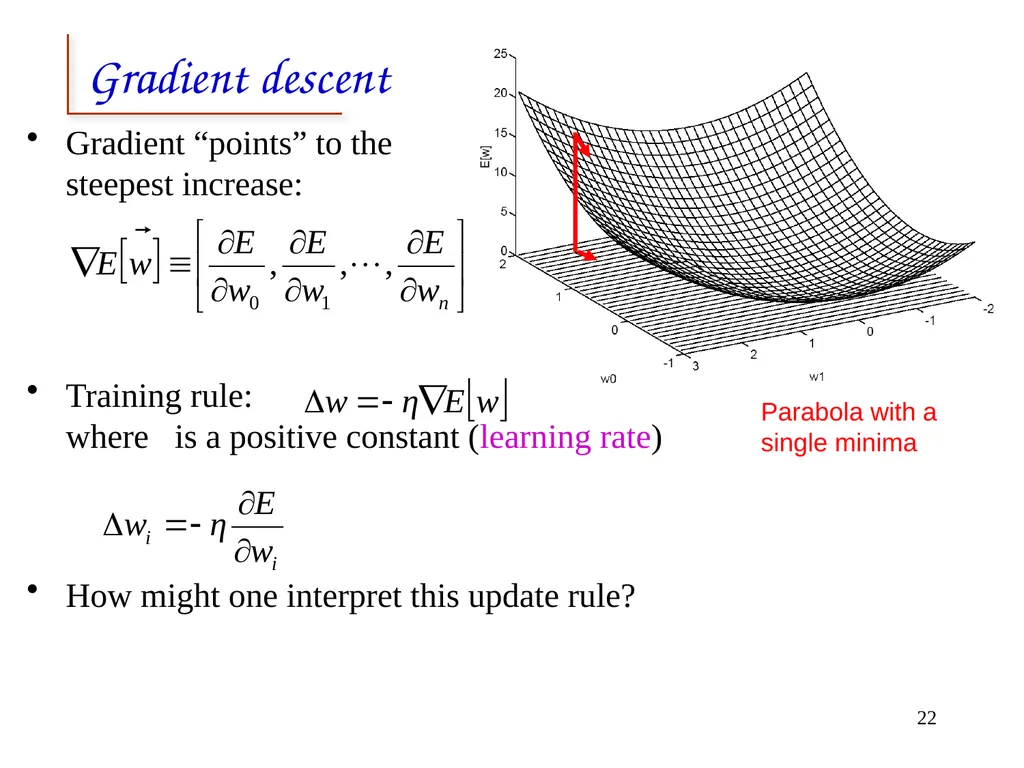
slide22. Gradient descent Gradient “points” to thesteepest increase:

Training rule:where  is a positive constant (learning rate)


How might one interpret this update rule? Parabola with a single minima 22<br>
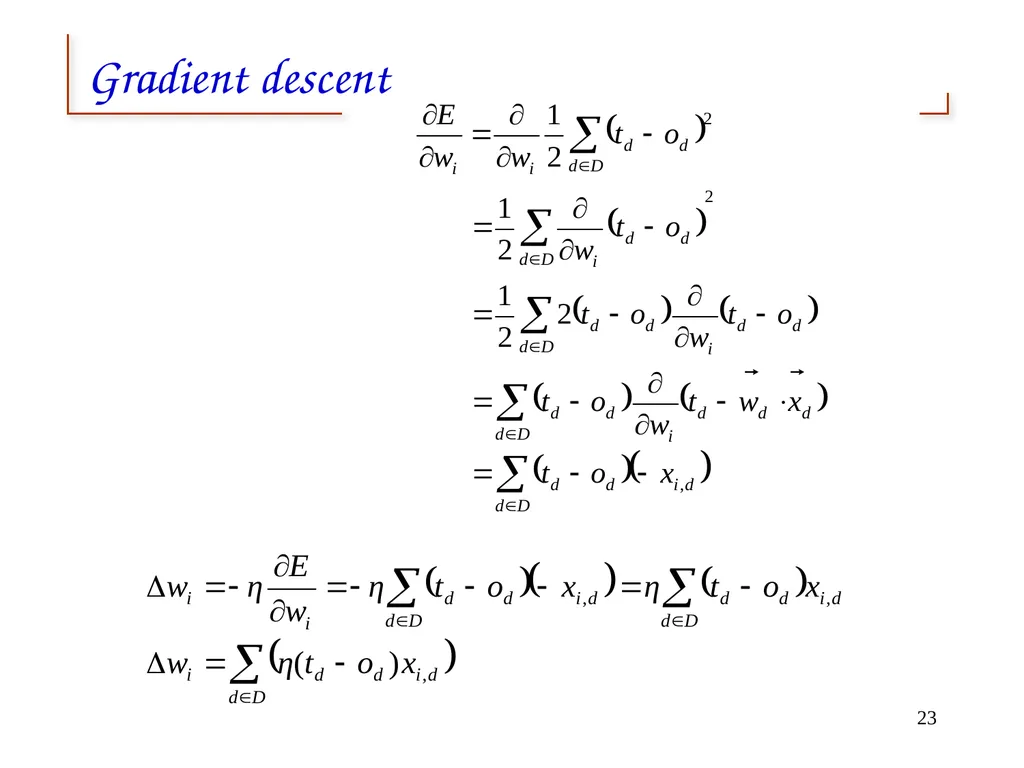
slide23. Gradient descent 23<br>
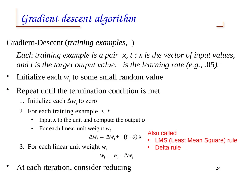
slide24. Gradient descent algorithm Gradient-Descent (training examples, )
Each training example is a pair x, t: x is the vector of input values, and t is the target output value.  is the learning rate (e.g., .05).
Initialize each wi to some small random value
Repeat until the termination condition is met
Initialize each Δwi to zero
For each training example x, t
Input x to the unit and compute the output o
For each linear unit weight wi Δwi ← Δwi +  (t - o) xi
For each linear unit weight wi wi ← wi + Δwi
At each iteration, consider reducing  24 Also called
LMS (Least Mean Square) rule
Delta rule<br>
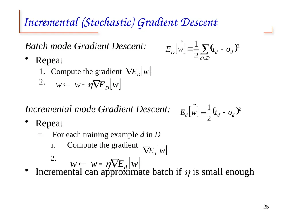
slide25. Incremental (Stochastic) Gradient Descent Batch mode Gradient Descent:
Repeat
Compute the gradient


Incremental mode Gradient Descent:
Repeat
For each training example d in D
Compute the gradient

Incremental can approximate batch if  is small enough 25<br>
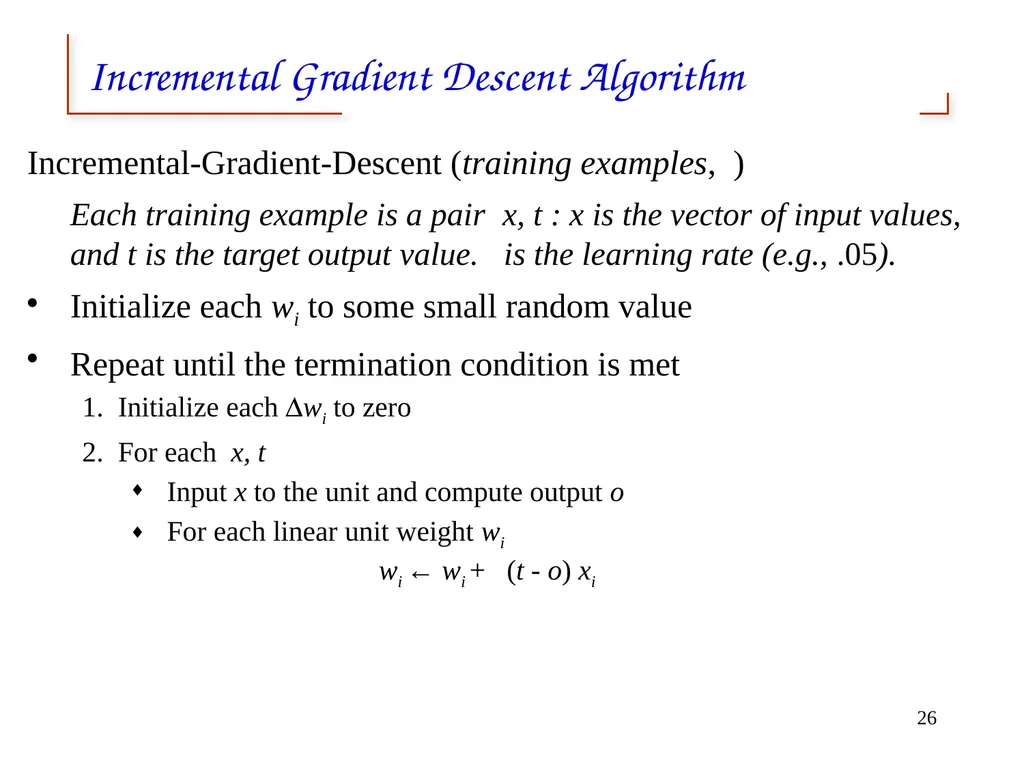
slide26. Incremental Gradient Descent Algorithm Incremental-Gradient-Descent (training examples, )
Each training example is a pair x, t: x is the vector of input values, and t is the target output value.  is the learning rate (e.g., .05).
Initialize each wi to some small random value
Repeat until the termination condition is met
Initialize each Dwi to zero
For each x, t
Input x to the unit and compute output o
For each linear unit weight wi wi ← wi +  (t - o) xi 26<br>
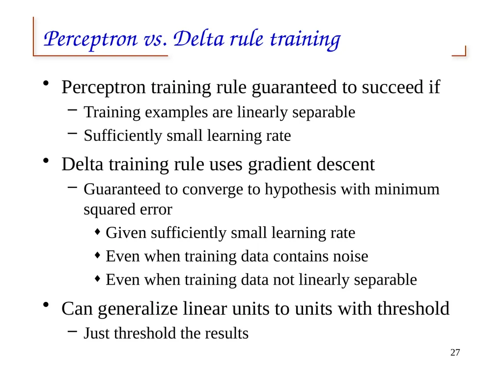
slide27. Perceptron vs. Delta rule training Perceptron training rule guaranteed to succeed if
Training examples are linearly separable
Sufficiently small learning rate
Delta training rule uses gradient descent
Guaranteed to converge to hypothesis with minimum squared error
Given sufficiently small learning rate
Even when training data contains noise
Even when training data not linearly separable
Can generalize linear units to units with threshold
Just threshold the results 27<br>
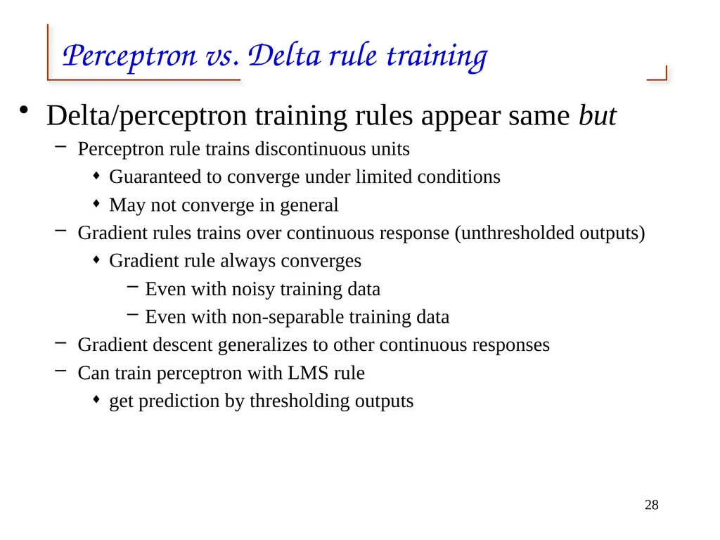
slide28. Perceptron vs. Delta rule training Delta/perceptron training rules appear same but
Perceptron rule trains discontinuous units
Guaranteed to converge under limited conditions
May not converge in general
Gradient rules trains over continuous response (unthresholded outputs)
Gradient rule always converges
Even with noisy training data
Even with non-separable training data
Gradient descent generalizes to other continuous responses
Can train perceptron with LMS rule
get prediction by thresholding outputs 28<br>
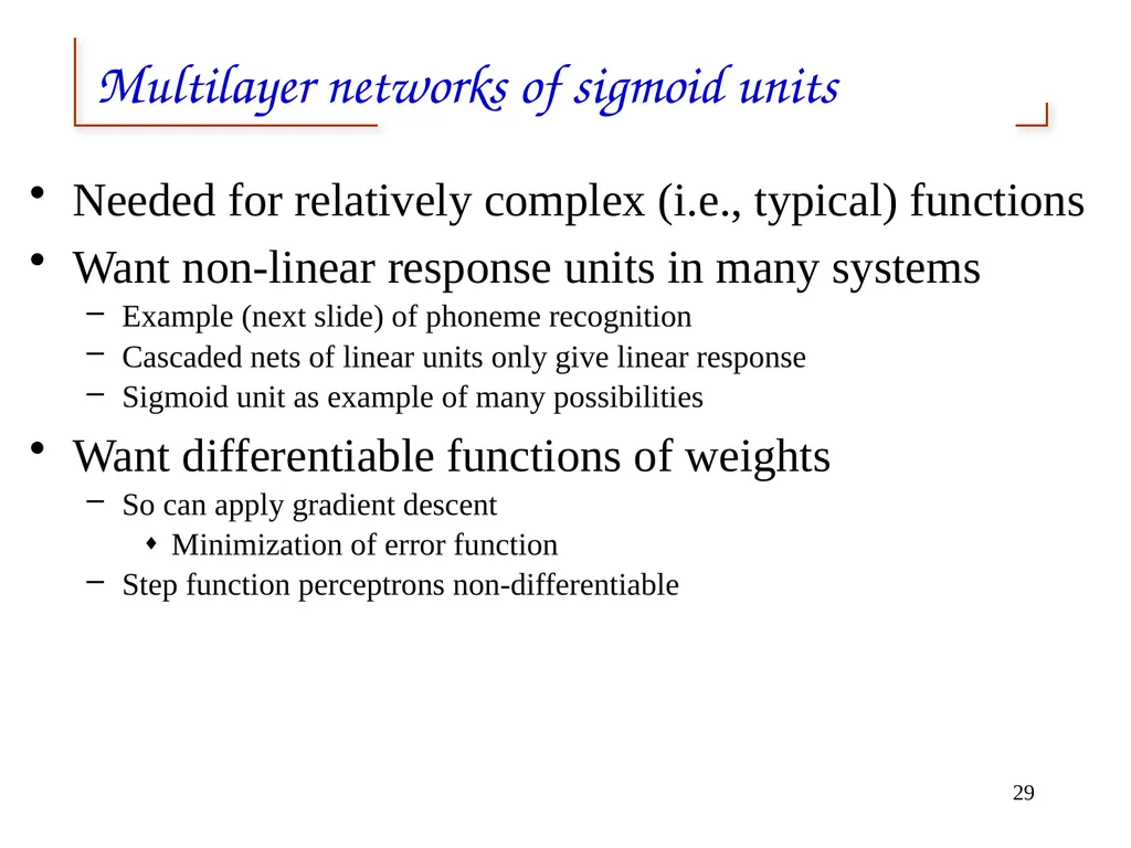
slide29. Multilayer networks of sigmoid units Needed for relatively complex (i.e., typical) functions
Want non-linear response units in many systems
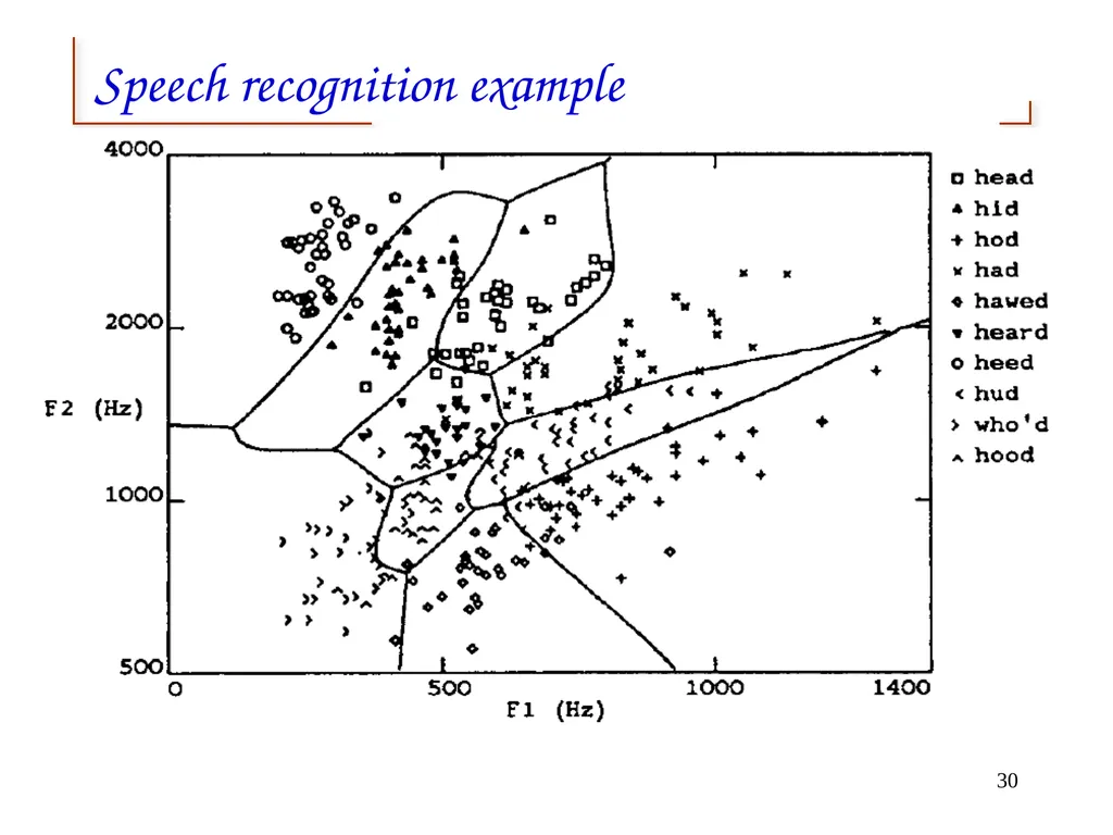
Example (next slide) of phoneme recognition
Cascaded nets of linear units only give linear response
Sigmoid unit as example of many possibilities
Want differentiable functions of weights
So can apply gradient descent
Minimization of error function
Step function perceptrons non-differentiable 29<br>
slide30. Speech recognition example 30<br>
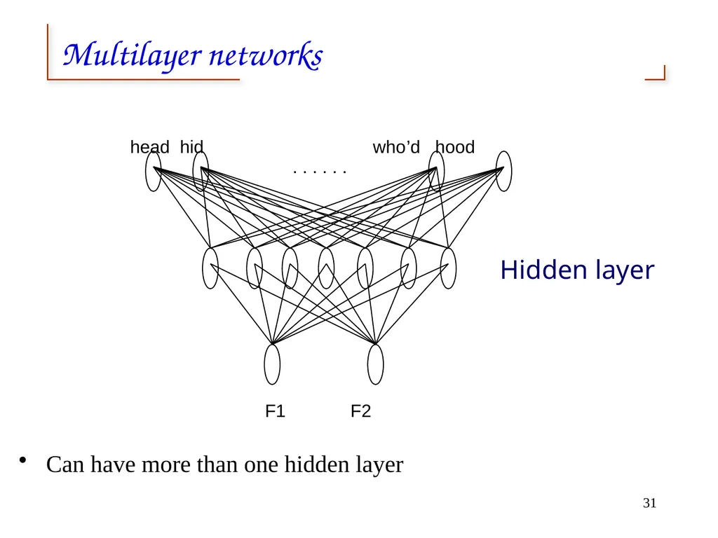
slide31. Multilayer networks F1 F2 . . . . . . head hid who’d hood Hidden layer Can have more than one hidden layer 31<br>
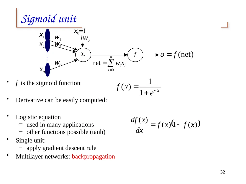
slide32. Sigmoid unit f is the sigmoid function

Derivative can be easily computed:

Logistic equation
used in many applications
other functions possible (tanh)
Single unit:
apply gradient descent rule
Multilayer networks: backpropagation x1 x2 xn w1 w2 wn :: x0=1 w0 S f 32<br>
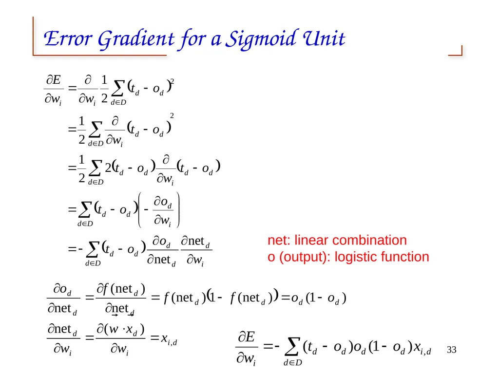
slide33. Error Gradient for a Sigmoid Unit 33 net: linear combination
o (output): logistic function<br>
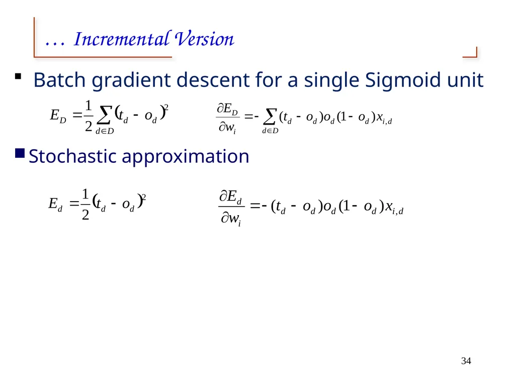
slide34. … Incremental Version Batch gradient descent for a single Sigmoid unit Stochastic approximation 34<br>
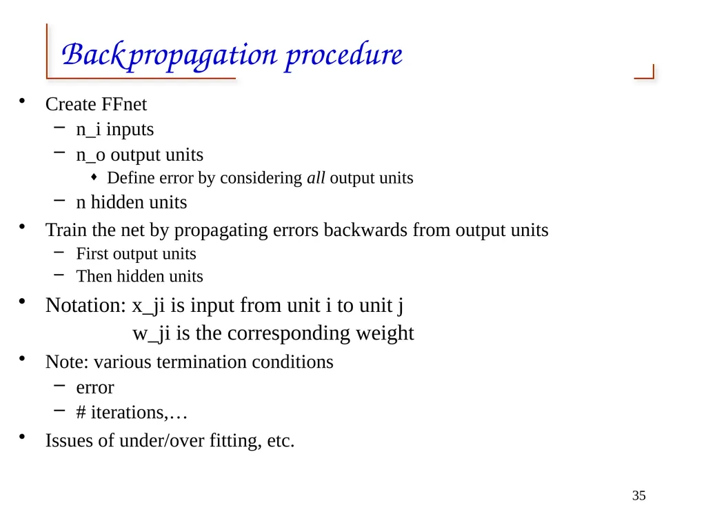
slide35. Backpropagation procedure Create FFnet
n_i inputs
n_o output units
Define error by considering all output units
n hidden units
Train the net by propagating errors backwards from output units
First output units
Then hidden units
Notation: x_ji is input from unit i to unit j
w_ji is the corresponding weight
Note: various termination conditions
error
# iterations,…
Issues of under/over fitting, etc. 35<br>
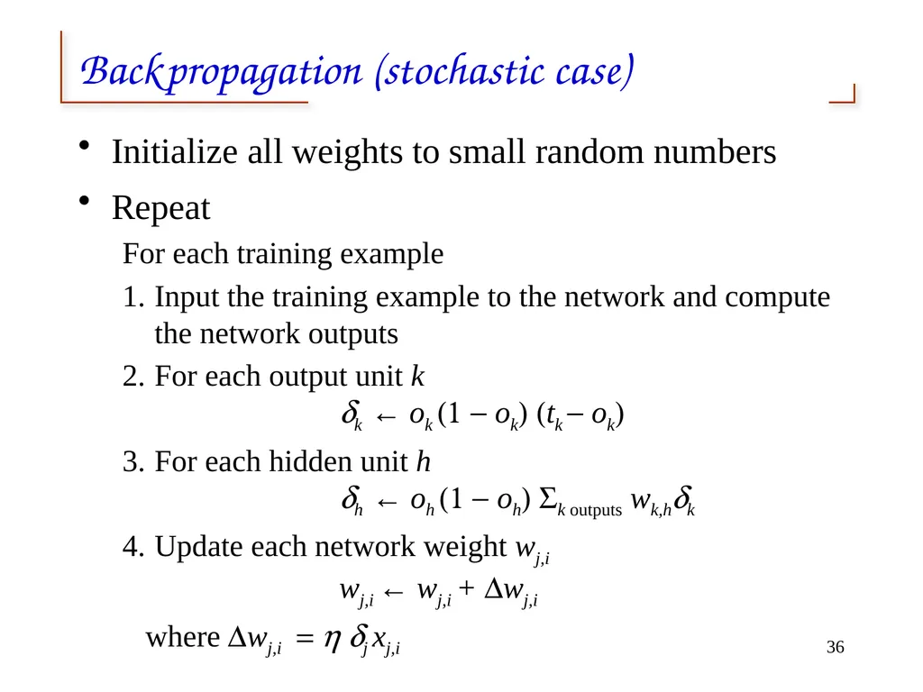
slide36. Backpropagation (stochastic case) Initialize all weights to small random numbers
Repeat
For each training example
Input the training example to the network and compute the network outputs
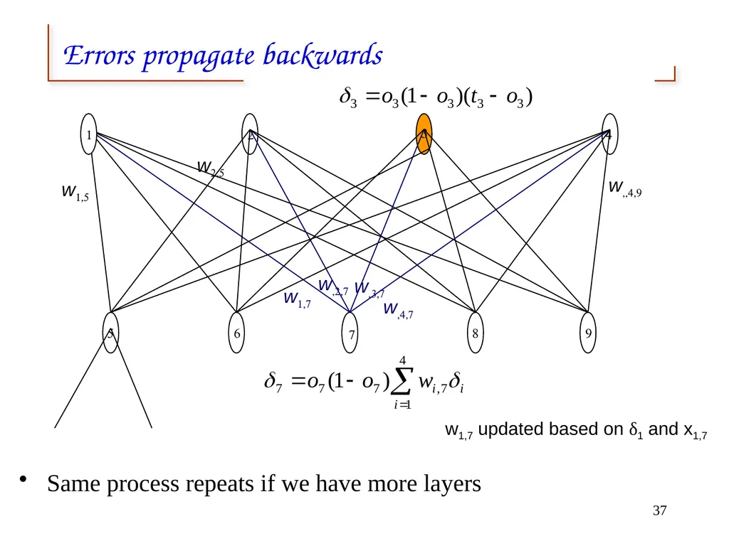
For each output unit k dk ← ok (1 - ok) (tk - ok)
For each hidden unit h dh ← oh (1 - oh) Skoutputs wk,hdk
Update each network weight wj,i wj,i ← wj,i + Dwj,i
where Dwj,i = h dj xj,i 36<br>
slide37. Errors propagate backwards Same process repeats if we have more layers 1 2 3 4 9 8 7 6 5 w,3,7 w,4,7 w,2,7 w1,7 w2,5 w1,5 w,,4,9 1 37 w1,7 updated based on δ1 and x1,7<br>
slide38. Properties of Backpropagation Easily generalized to arbitrary directed (acyclic) graphs
Backpropagate errors through the different layers
Training is slow but applying network after training is fast 38<br>
slide39. Convergence of Backpropagation Convergence
Training can take thousands of iterations → slow!
Gradient descent over entire network weight vector
Speed up using small initial values of weights:
Linear response initially
Generally will find local minimum
Typically can find good approximation to global minimum
Solutions to local minimum trap problem
Stochastic gradient descent
Can run multiple times
Over different initial weights
Committee of networks
Can modify to find better approximation to global minimum
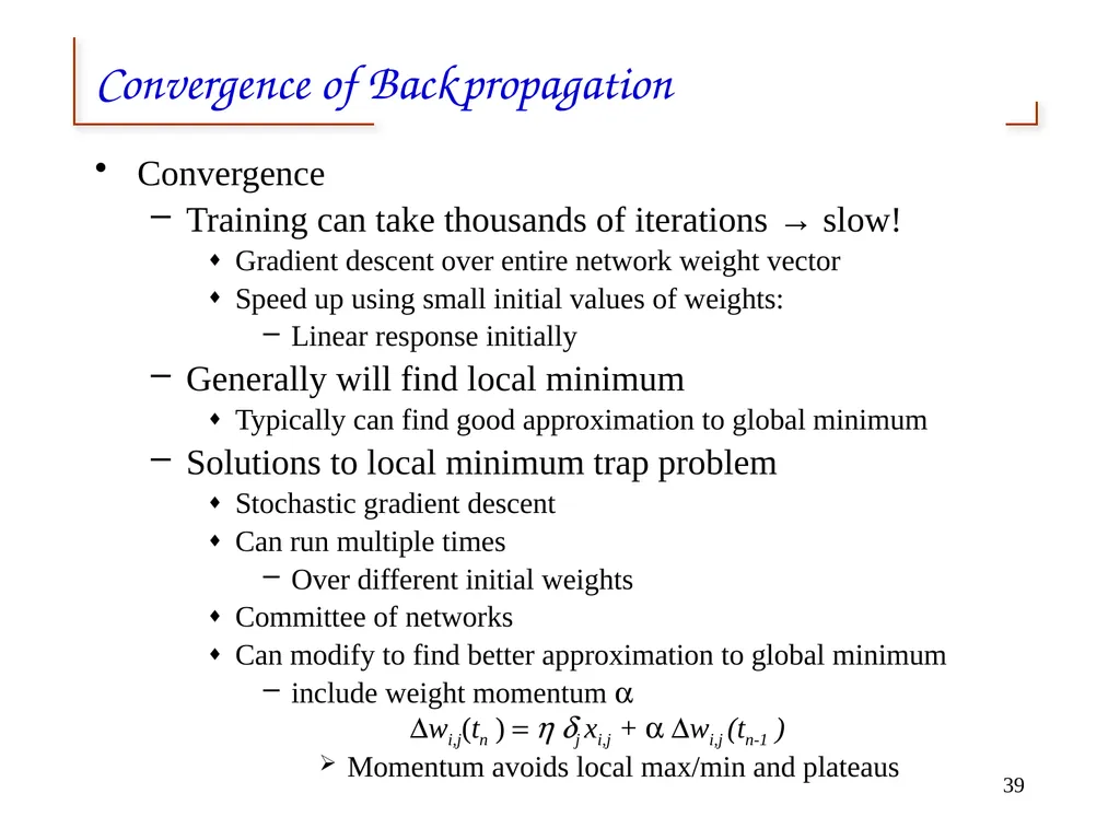
include weight momentum a  Dwi,j(tn ) = h dj xi,j + a Dwi,j (tn-1 )
Momentum avoids local max/min and plateaus 39<br>
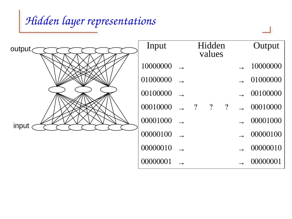
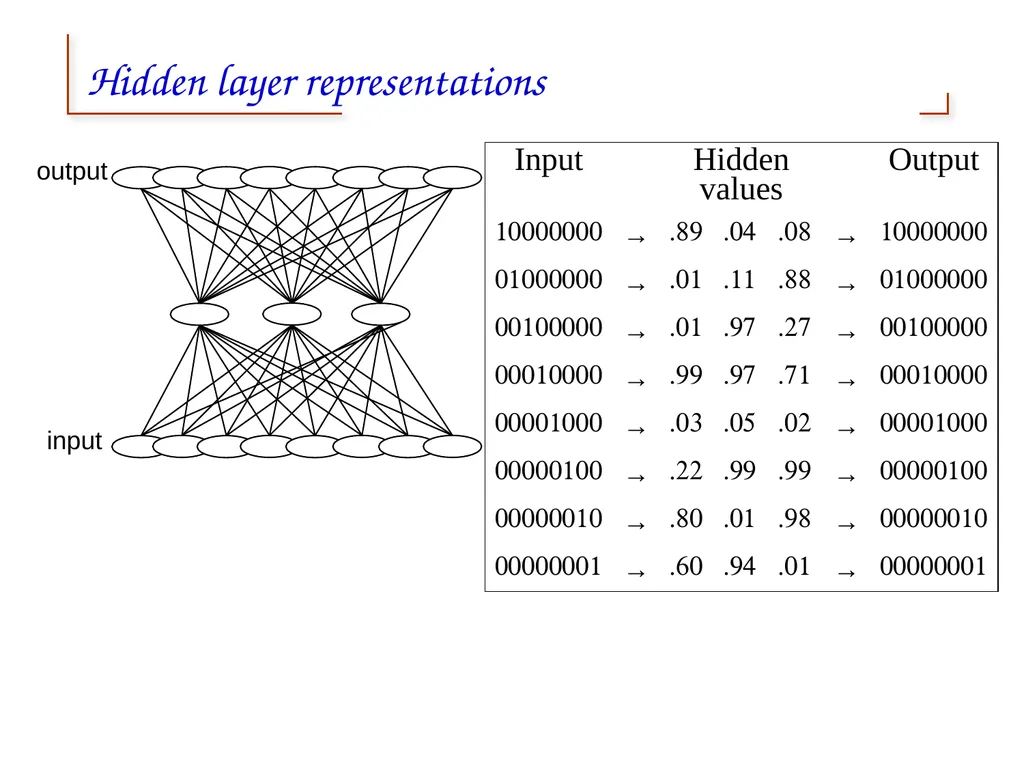
slide40. Example of learning a simple function Learn to recognize 8 simple inputs
Interest in how to interpret hidden units
System learns binary representation!
Trained with
initial w_i between –0.1, +0.1,
eta=0.3
5000 iterations (most change in first 50%)
Target output values:
.1 for 0
.9 for 1 40<br>
slide41. Hidden layer representations input output<br>
slide42. Hidden layer representations input output<br>
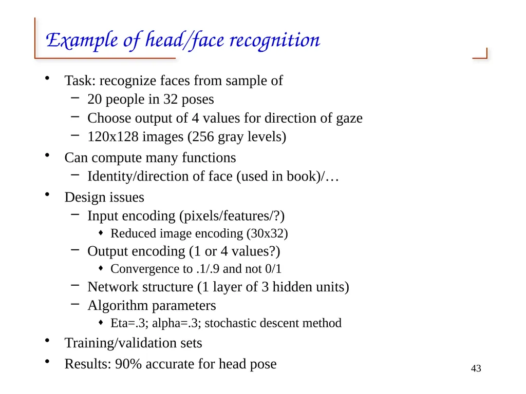
slide43. Example of head/face recognition Task: recognize faces from sample of
20 people in 32 poses
Choose output of 4 values for direction of gaze
120x128 images (256 gray levels)
Can compute many functions
Identity/direction of face (used in book)/…
Design issues
Input encoding (pixels/features/?)
Reduced image encoding (30x32)
Output encoding (1 or 4 values?)
Convergence to .1/.9 and not 0/1
Network structure (1 layer of 3 hidden units)
Algorithm parameters
Eta=.3; alpha=.3; stochastic descent method
Training/validation sets
Results: 90% accurate for head pose 43<br>
slide44. Some issues with ANNs Interpretation of hidden units
Hidden units “discover” new patterns/regularities
Often difficult to interpret
Overfitting
Expressiveness
Generalization to different classes of functions 44<br>
slide45. Dealing with overfitting Complex decision surface
Divide sample into
Training set
Validation set
Solutions
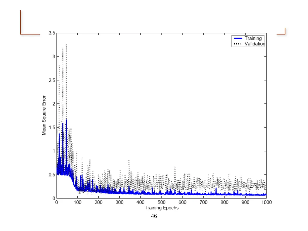
Return to weight set occurring near minimum over validation set
Prevent weights from becoming too large
Reduce weights by (small) proportionate amount at each iteration 45<br>
slide46. 46<br>
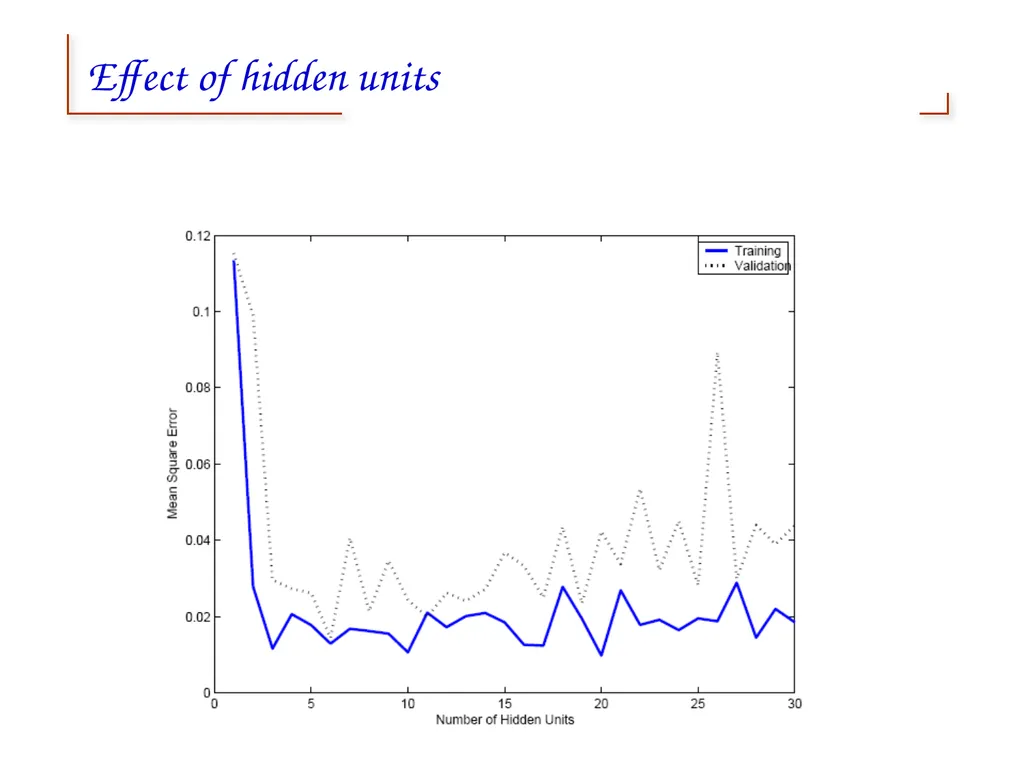
slide47. 47 Effect of hidden units<br>
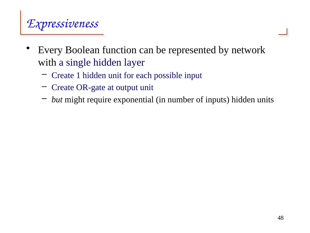
slide48. Expressiveness Every Boolean function can be represented by network with a single hidden layer
Create 1 hidden unit for each possible input
Create OR-gate at output unit
but might require exponential (in number of inputs) hidden units 48<br>
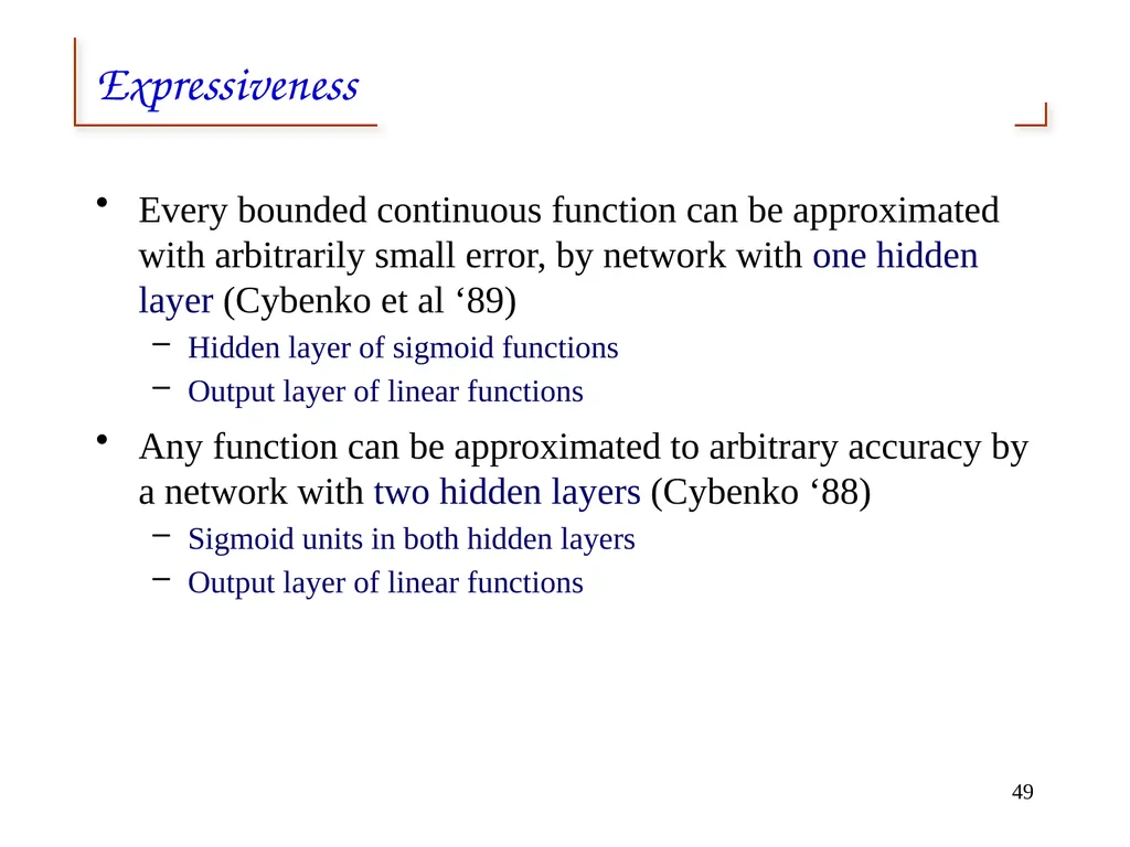
slide49. Expressiveness Every bounded continuous function can be approximated with arbitrarily small error, by network with one hidden layer (Cybenko et al ‘89)
Hidden layer of sigmoid functions
Output layer of linear functions
Any function can be approximated to arbitrary accuracy by a network with two hidden layers (Cybenko ‘88)
Sigmoid units in both hidden layers
Output layer of linear functions 49<br>
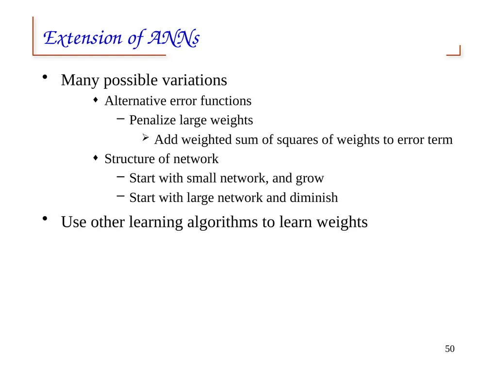
slide50. Extension of ANNs Many possible variations
Alternative error functions
Penalize large weights
Add weighted sum of squares of weights to error term
Structure of network
Start with small network, and grow
Start with large network and diminish
Use other learning algorithms to learn weights 50<br>
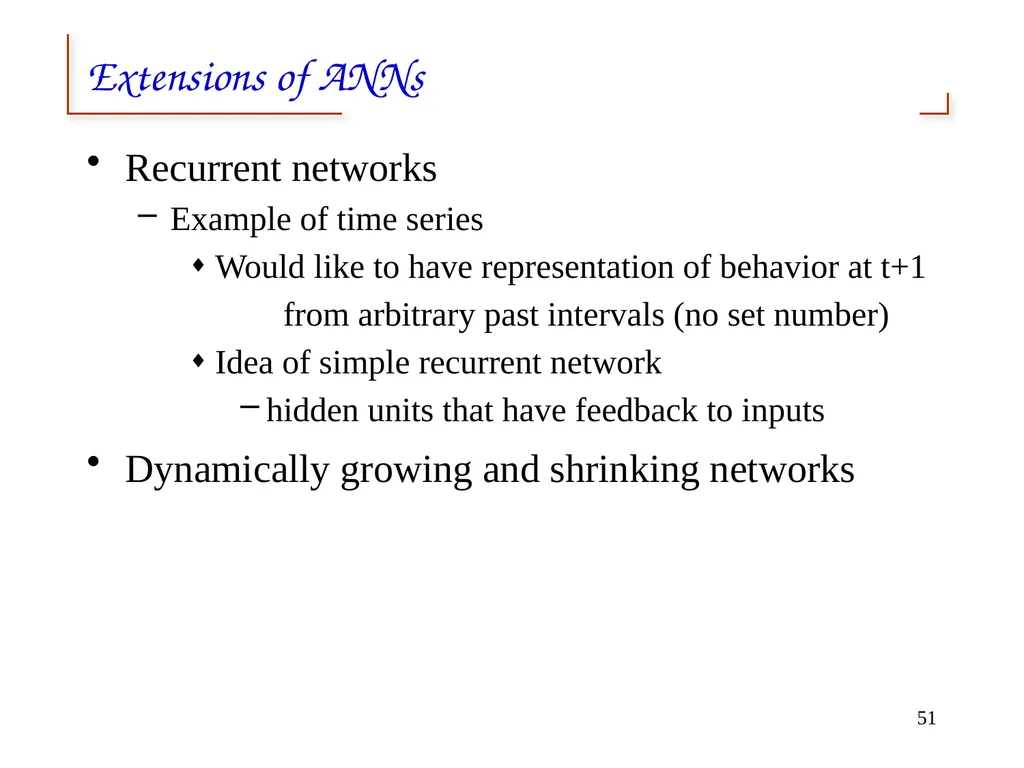
slide51. Extensions of ANNs Recurrent networks
Example of time series
Would like to have representation of behavior at t+1
from arbitrary past intervals (no set number)
Idea of simple recurrent network
hidden units that have feedback to inputs
Dynamically growing and shrinking networks 51<br>
slide52. Inductive bias of Backpropagation Smooth interpolation between data points 52<br>
slide53. Summary Practical method for learning continuous functions over continuous and discrete attributes
Robust to noise
Slow to train but fast afterwards
Gradient descent search over space of weights
Overfitting can be a problem
Hidden layers can invent new features 53<br>
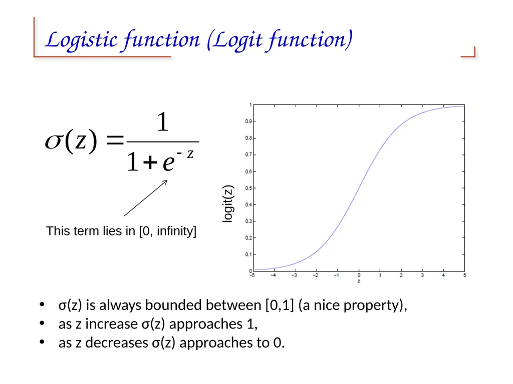
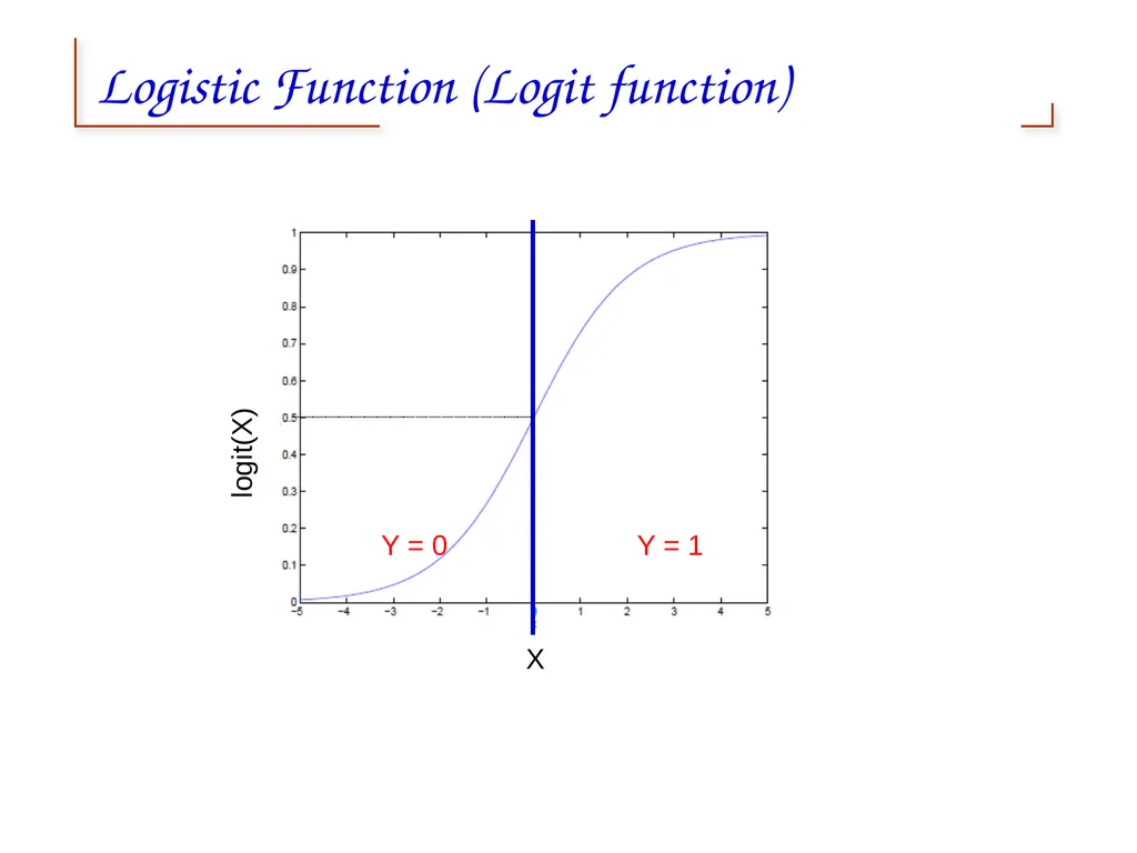
slide54. Logistic function (Logit function) z logit(z) σ(z) is always bounded between [0,1] (a nice property),
as z increase σ(z) approaches 1,
as z decreases σ(z) approaches to 0. This term lies in [0, infinity]<br>
slide55. Segway: Logistic regression Logistic regression is often used because the relationship between the dependent discrete variable and a predictor is non-linear
Example: the probability of heart disease changes very little with a ten-point difference among people with low-blood pressure, but a ten point change can mean a drastic change in the probability of heart disease in people with high blood-pressure.<br>
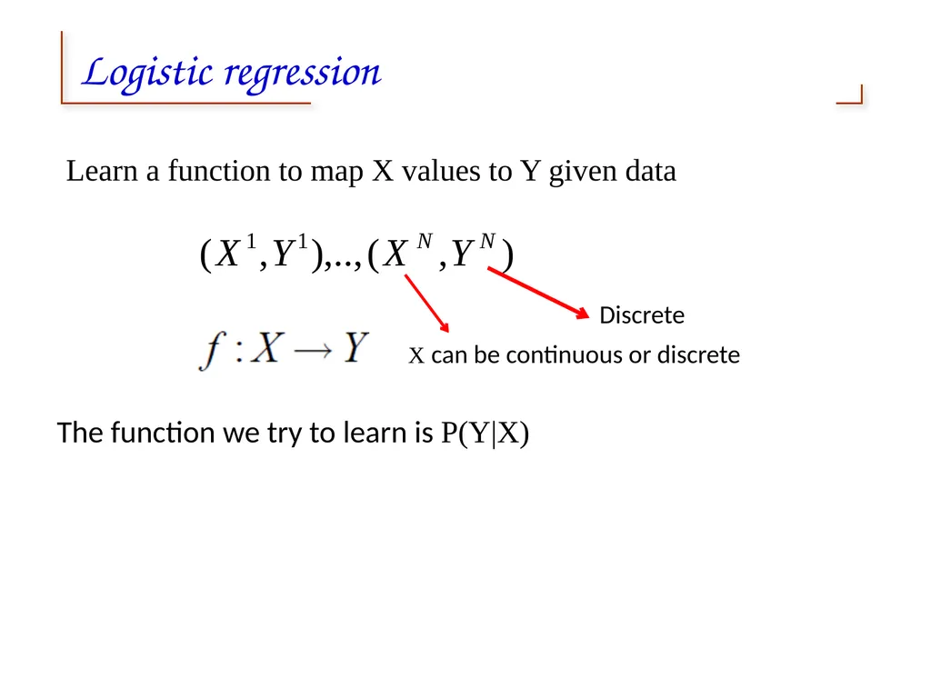
slide56. Logistic regression Learn a function to map X values to Y given data The function we try to learn is P(Y|X) X can be continuous or discrete Discrete<br>
slide57. Logistic regression (Classification)<br>
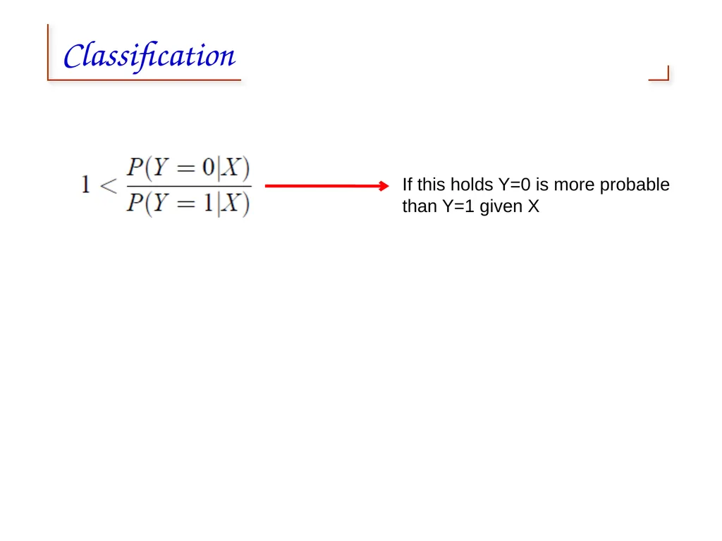
slide58. Classification If this holds Y=0 is more probable
than Y=1 given X<br>
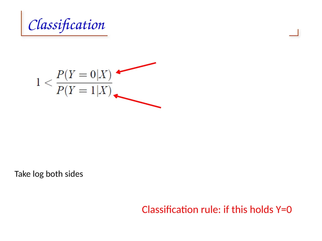
slide59. Classification Take log both sides Classification rule: if this holds Y=0<br>
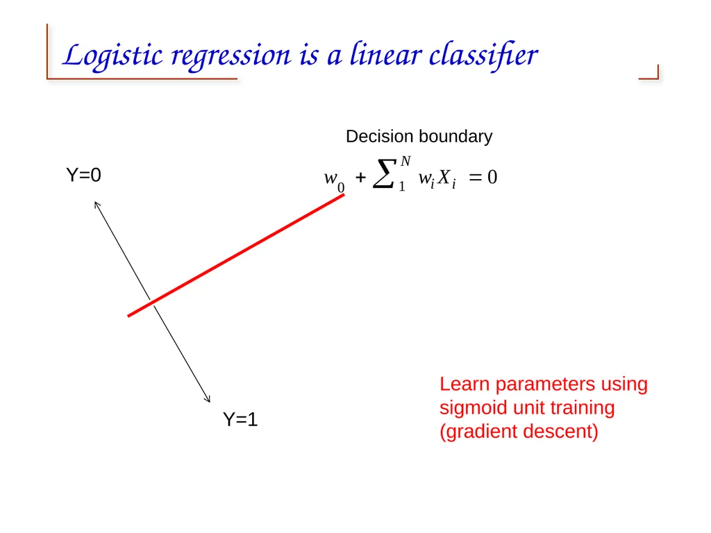
slide60. Logistic regression is a linear classifier Y=0 Y=1 Decision boundary Learn parameters using sigmoid unit training (gradient descent)<br>
slide61. Logistic Function (Logit function) z logit(X) Y = 0 Y = 1 X<br>