Can a brain-imaging foundation model see

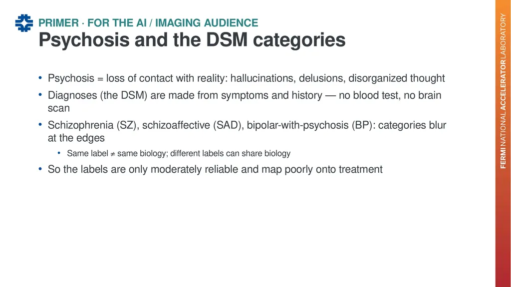
Psychosis = loss of contact with reality: hallucinations, delusions, disorganized thought
Diagnoses (the DSM) are made from symptoms and history — no blood test, no brain scan
Schizophrenia (SZ), schizoaffective (SAD), bipolar-with-psychosis (BP): categories blur at the edges
Same label ≠ same biology; different labels can share biology
So the labels are only moderately reliable and map poorly onto treatment Psychosis and the DSM categories PRIMER · FOR THE AI / IMAGING AUDIENCE<br>

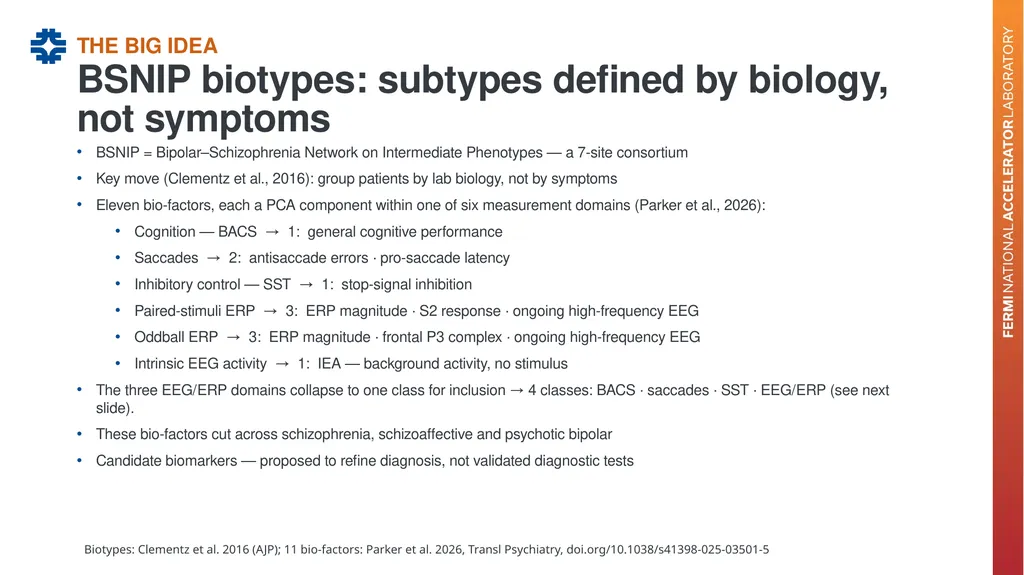
BSNIP = Bipolar–Schizophrenia Network on Intermediate Phenotypes — a 7-site consortium
Key move (Clementz et al., 2016): group patients by lab biology, not by symptoms
Eleven bio-factors, each a PCA component within one of six measurement domains (Parker et al., 2026):
Cognition — BACS → 1: general cognitive performance
Saccades → 2: antisaccade errors · pro-saccade latency
Inhibitory control — SST → 1: stop-signal inhibition
Paired-stimuli ERP → 3: ERP magnitude · S2 response · ongoing high-frequency EEG
Oddball ERP → 3: ERP magnitude · frontal P3 complex · ongoing high-frequency EEG
Intrinsic EEG activity → 1: IEA — background activity, no stimulus
The three EEG/ERP domains collapse to one class for inclusion → 4 classes: BACS · saccades · SST · EEG/ERP (see next slide).
These bio-factors cut across schizophrenia, schizoaffective and psychotic bipolar
Candidate biomarkers — proposed to refine diagnosis, not validated diagnostic tests BSNIP biotypes: subtypes defined by biology, not symptoms THE BIG IDEA Biotypes: Clementz et al. 2016 (AJP); 11 bio-factors: Parker et al. 2026, Transl Psychiatry, doi.org/10.1038/s41398-025-03501-5<br>

11 'bio-factors' from 4 biomarker classes: Cognition (BACS) · Saccades (antisaccade, latency) · Stop-signal (SST) · EEG/ERP (paired-stimulus + oddball ERPs, intrinsic activity).
Each = a PCA component within its class, age/sex-adjusted and standardized (mean 0, SD 1). Parker 2025 extended 9→11 (added intrinsic activity; split paired vs oddball).
Inclusion: available data on a majority of the 4 classes (≥3 of 4). Missing bio-factors are regression-imputed for the scores, but biotype assignment uses only the available dimensions.
k-means on psychosis cases → BT1 / BT2 / BT3 (three clusters — gap statistic + 23 NBclust estimators).
Nearest-centroid; individual-case assignment stable only with >1,000 probands (Rand index). Gradient: BT1 most impaired → BT3 nearest normal biology and cognition.
Healthy controls are NOT a biotype — the normative reference (used to age-adjust and standardize); clustering runs on psychosis cases only.
Geometry of the separation: the 11 bio-factors are independent axes, but pooled subjects effectively occupy only a ~6-D subspace — and just 3 dimensions sort them into groups (Parker's canonical 'Pattern 1/2/3').
Why 3: the four centroids — BT1, BT2, BT3 + controls — form a tetrahedron; four non-coplanar points (non-zero volume) span a 3-D affine subspace, its 6 edge-lengths the between-group distances.
DSM SZ/SAD/BP are not neurobiologically distinct — the biology sorts along these axes instead (Parker 2025). Biotypes, biofactors, inclusion, and controls METHOD · HOW BIOTYPES ARE BUILT Candidate biomarkers vs. validated tests — APA, The Future of the DSM (2026): doi.org/10.1176/appi.ajp.20250877<br>

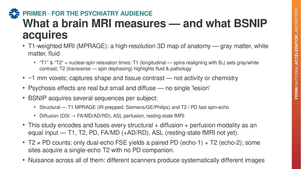
T1-weighted MRI (MPRAGE): a high-resolution 3D map of anatomy — gray matter, white matter, fluid
“T1” & “T2” = nuclear-spin relaxation times: T1 (longitudinal — spins realigning with B₀) sets gray/white contrast; T2 (transverse — spin dephasing) highlights fluid & pathology
~1 mm voxels; captures shape and tissue contrast — not activity or chemistry
Psychosis effects are real but small and diffuse — no single 'lesion'
BSNIP acquires several sequences per subject:
Structural — T1 MPRAGE (IR-prepped; Siemens/GE/Philips) and T2 / PD fast spin-echo
Diffusion (DSI → FA/MD/AD/RD), ASL perfusion, resting-state fMRI
This study encodes and fuses every structural + diffusion + perfusion modality as an equal input — T1, T2, PD, FA/MD (+AD/RD), ASL (resting-state fMRI not yet).
T2 ≠ PD counts: only dual-echo FSE yields a paired PD (echo-1) + T2 (echo-2); some sites acquire a single-echo T2 with no PD companion.
Nuisance across all of them: different scanners produce systematically different images What a brain MRI measures — and what BSNIP acquires PRIMER · FOR THE PSYCHIATRY AUDIENCE<br>

Our approach: a frozen imaging foundation model 02<br>

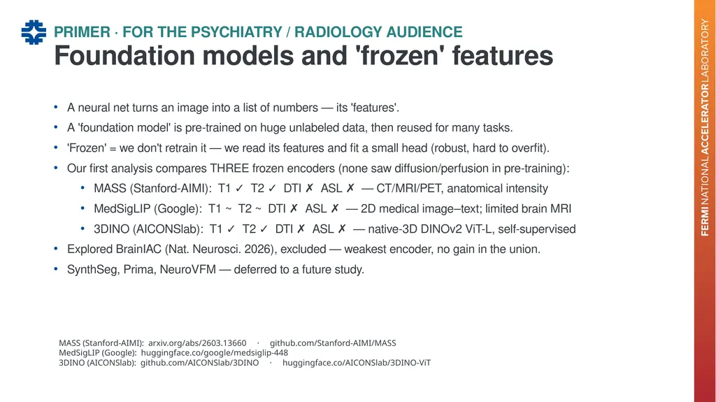
A neural net turns an image into a list of numbers — its 'features'.
A 'foundation model' is pre-trained on huge unlabeled data, then reused for many tasks.
'Frozen' = we don't retrain it — we read its features and fit a small head (robust, hard to overfit).
Our first analysis compares THREE frozen encoders (none saw diffusion/perfusion in pre-training):
MASS (Stanford-AIMI): T1 ✓ T2 ✓ DTI ✗ ASL ✗ — CT/MRI/PET, anatomical intensity
MedSigLIP (Google): T1 ~ T2 ~ DTI ✗ ASL ✗ — 2D medical image–text; limited brain MRI
3DINO (AICONSlab): T1 ✓ T2 ✓ DTI ✗ ASL ✗ — native-3D DINOv2 ViT-L, self-supervised
Explored BrainIAC (Nat. Neurosci. 2026), excluded — weakest encoder, no gain in the union.
SynthSeg, Prima, NeuroVFM — deferred to a future study. Foundation models and 'frozen' features PRIMER · FOR THE PSYCHIATRY / RADIOLOGY AUDIENCE MASS (Stanford-AIMI): arxiv.org/abs/2603.13660 · github.com/Stanford-AIMI/MASS
MedSigLIP (Google): huggingface.co/google/medsiglip-448
3DINO (AICONSlab): github.com/AICONSlab/3DINO · huggingface.co/AICONSlab/3DINO-ViT<br>

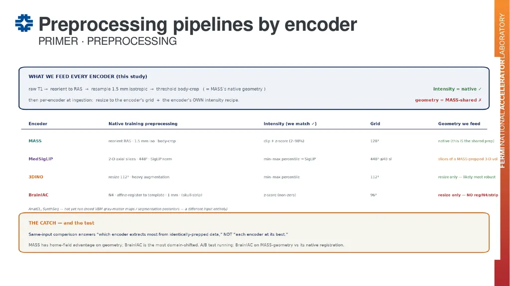
Preprocessing pipelines by encoder PRIMER · PREPROCESSING<br>

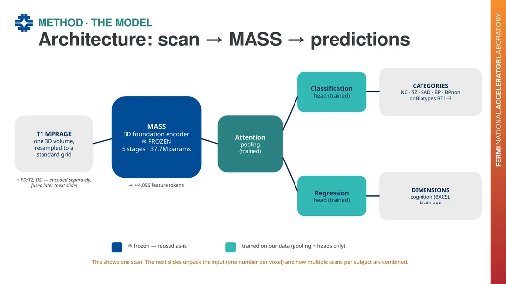
Architecture: scan → MASS → predictions METHOD · THE MODEL T1 MPRAGE
one 3D volume,
resampled to a
standard grid + PD/T2, DSI — encoded separately, fused later (next slide) MASS
3D foundation encoder
❄ FROZEN
5 stages · 37.7M params → ≈4,096 feature tokens Attention
pooling
(trained) Classification
head (trained) CATEGORIES
NC · SZ · SAD · BP · BPnon
or Biotypes BT1–3 Regression
head (trained) DIMENSIONS
cognition (BACS),
brain age ❄ frozen — reused as-is trained on our data (pooling + heads only) This shows one scan. The next slides unpack the input (one number per voxel) and how multiple scans per subject are combined.<br>

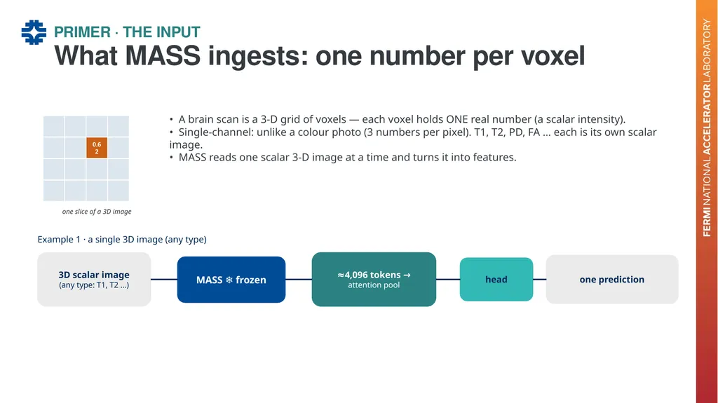
What MASS ingests: one number per voxel PRIMER · THE INPUT 0.62 one slice of a 3D image • A brain scan is a 3-D grid of voxels — each voxel holds ONE real number (a scalar intensity).
• Single-channel: unlike a colour photo (3 numbers per pixel). T1, T2, PD, FA … each is its own scalar image.
• MASS reads one scalar 3-D image at a time and turns it into features. Example 1 · a single 3D image (any type) 3D scalar image
(any type: T1, T2 …) MASS ❄ frozen ≈4,096 tokens →
attention pool head one prediction<br>

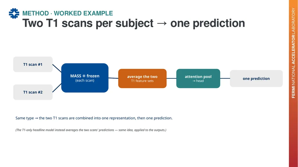
Two T1 scans per subject → one prediction METHOD · WORKED EXAMPLE T1 scan #1 T1 scan #2 MASS ❄ frozen
(each scan) average the two
T1 feature sets attention pool
→ head one prediction Same type → the two T1 scans are combined into one representation, then one prediction. (The T1-only headline model instead averages the two scans' predictions — same idea, applied to the outputs.)<br>

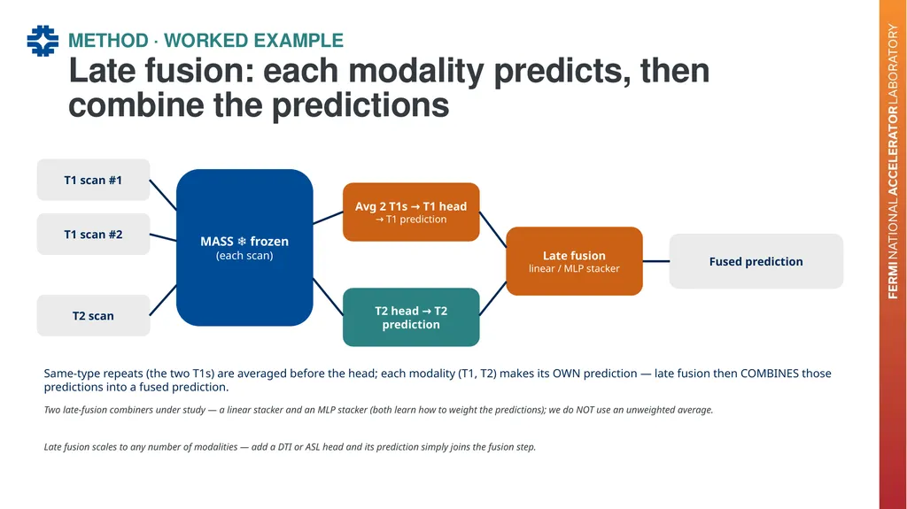
Late fusion: each modality predicts, then combine the predictions METHOD · WORKED EXAMPLE T1 scan #1 T1 scan #2 T2 scan MASS ❄ frozen
(each scan) Avg 2 T1s → T1 head
→ T1 prediction T2 head → T2 prediction Late fusion
linear / MLP stacker Fused prediction Same-type repeats (the two T1s) are averaged before the head; each modality (T1, T2) makes its OWN prediction — late fusion then COMBINES those predictions into a fused prediction. Two late-fusion combiners under study — a linear stacker and an MLP stacker (both learn how to weight the predictions); we do NOT use an unweighted average. Late fusion scales to any number of modalities — add a DTI or ASL head and its prediction simply joins the fusion step.<br>

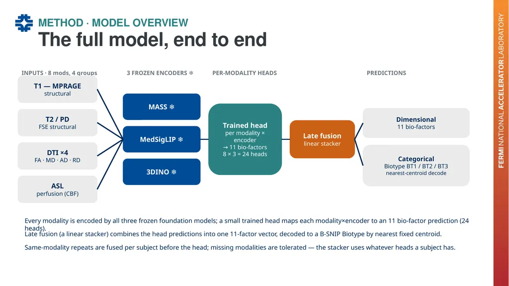
The full model, end to end METHOD · MODEL OVERVIEW INPUTS · 8 mods, 4 groups 3 FROZEN ENCODERS ❄ PER-MODALITY HEADS PREDICTIONS T1 — MPRAGE
structural T2 / PD
FSE structural DTI ×4
FA · MD · AD · RD ASL
perfusion (CBF) MASS ❄ MedSigLIP ❄ 3DINO ❄ Trained head
per modality × encoder
→ 11 bio-factors
8 × 3 = 24 heads Late fusion
linear stacker Dimensional
11 bio-factors Categorical
Biotype BT1 / BT2 / BT3
nearest-centroid decode Every modality is encoded by all three frozen foundation models; a small trained head maps each modality×encoder to an 11 bio-factor prediction (24 heads). Late fusion (a linear stacker) combines the head predictions into one 11-factor vector, decoded to a B-SNIP Biotype by nearest fixed centroid. Same-modality repeats are fused per subject before the head; missing modalities are tolerated — the stacker uses whatever heads a subject has.<br>

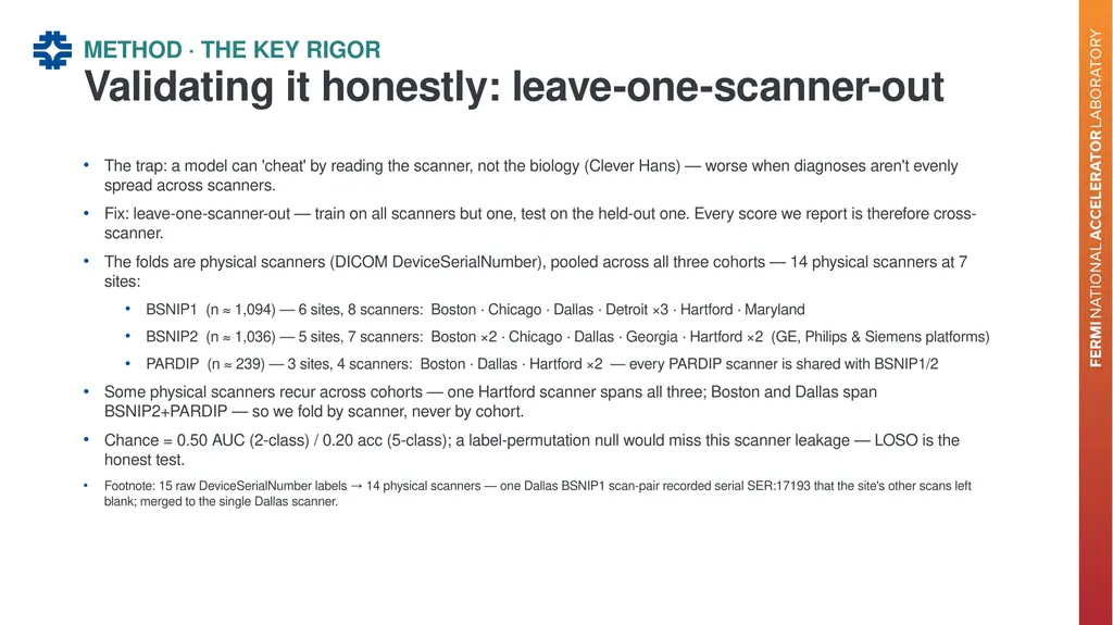
The trap: a model can 'cheat' by reading the scanner, not the biology (Clever Hans) — worse when diagnoses aren't evenly spread across scanners.
Fix: leave-one-scanner-out — train on all scanners but one, test on the held-out one. Every score we report is therefore cross-scanner.
The folds are physical scanners (DICOM DeviceSerialNumber), pooled across all three cohorts — 14 physical scanners at 7 sites:
BSNIP1 (n ≈ 1,094) — 6 sites, 8 scanners: Boston · Chicago · Dallas · Detroit ×3 · Hartford · Maryland
BSNIP2 (n ≈ 1,036) — 5 sites, 7 scanners: Boston ×2 · Chicago · Dallas · Georgia · Hartford ×2 (GE, Philips & Siemens platforms)
PARDIP (n ≈ 239) — 3 sites, 4 scanners: Boston · Dallas · Hartford ×2 — every PARDIP scanner is shared with BSNIP1/2
Some physical scanners recur across cohorts — one Hartford scanner spans all three; Boston and Dallas span BSNIP2+PARDIP — so we fold by scanner, never by cohort.
Chance = 0.50 AUC (2-class) / 0.20 acc (5-class); a label-permutation null would miss this scanner leakage — LOSO is the honest test.
Footnote: 15 raw DeviceSerialNumber labels → 14 physical scanners — one Dallas BSNIP1 scan-pair recorded serial SER:17193 that the site's other scans left blank; merged to the single Dallas scanner. Validating it honestly: leave-one-scanner-out METHOD · THE KEY RIGOR<br>

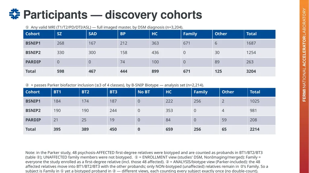
Participants — discovery cohorts Note: in the Parker study, 48 psychosis-AFFECTED first-degree relatives were biotyped and are counted as probands in BT1/BT2/BT3 (table ②); UNAFFECTED family members were not biotyped. ① = ENROLLMENT view (studies' DSM, NonImaging/merged): Family = everyone the study enrolled as a first-degree relative (incl. those 48 affected). ② = ANALYSIS/biotype view (Parker-included): the 48 affected relatives move into BT1/BT2/BT3 with the other probands; only NON-biotyped (unaffected) relatives remain in ②'s Family. So a subject is Family in ① yet a biotyped proband in ② — different views, each counting every subject exactly once (no double-count). SZ/SAD/BP = psychotic probands by DSM; HC = control; Other = non-psychotic BP + unresolved. From master_images_deduped.csv. ① Any valid MRI (T1/T2/PD/DTI/ASL) — full imaged master, by DSM diagnosis (n=3,204). ② + passes Parker biofactor inclusion (≥3 of 4 classes), by B-SNIP Biotype — analysis set (n=2,214).<br>

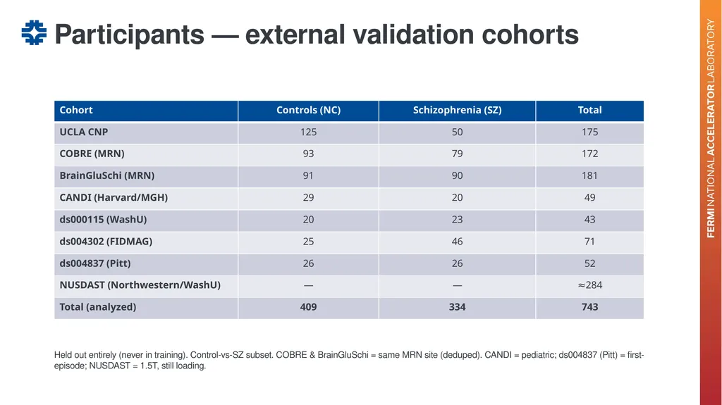
Held out entirely (never in training). Control-vs-SZ subset. COBRE & BrainGluSchi = same MRN site (deduped). CANDI = pediatric; ds004837 (Pitt) = first-episode; NUSDAST = 1.5T, still loading. Participants — external validation cohorts<br>

What we found 03<br>

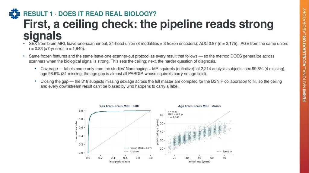
SEX from brain MRI, leave-one-scanner-out, 24-head union (8 modalities × 3 frozen encoders): AUC 0.97 (n = 2,175). AGE from the same union: r = 0.83 (≈7-yr error, n = 1,940).
Same frozen features and the same leave-one-scanner-out protocol as every result that follows — so the method DOES generalize across scanners when the biological signal is strong. This sets the ceiling; next, the harder question of diagnosis.
Coverage — labels come only from the studies' NonImaging + MR squirrels (definitive): of 2,214 analysis subjects, sex 99.8% (4 missing), age 98.6% (31 missing; the age gap is almost all PARDIP, whose squirrels carry no age field).
Closing the gap — the 318 subjects missing sex/age across the full master are compiled for the BSNIP collaboration to fill, so the ceiling and every downstream result can't be biased by who happens to carry a label. First, a ceiling check: the pipeline reads strong signals RESULT 1 · DOES IT READ REAL BIOLOGY?<br>

5-way DSM diagnosis, physical-scanner LOSO: macro-OvR AUC 0.54 — barely above chance (0.50)
Same features, biology-based biotypes (BT1–BT3): AUC 0.59 — above chance and above DSM
NC-vs-any-psychosis on the same folds reaches 0.67 — the coarse split transfers, the fine DSM subtypes don't
Biology-defined subtypes are more brain-separable than symptom-defined labels
Against the sex/age ceiling, this says the categories overlap — the biology carries the signal DSM categories don't transfer across scanners — biotypes do better RESULT 2<br>

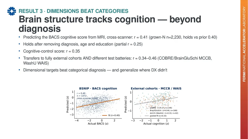
Predicting the BACS cognitive score from MRI, cross-scanner: r = 0.41 (grown-N n=2,230, holds vs prior 0.40)
Holds after removing diagnosis, age and education (partial r = 0.25)
Cognitive-control score: r = 0.35
Transfers to fully external cohorts AND different test batteries: r ≈ 0.34–0.46 (COBRE/BrainGluSchi MCCB, WashU WAIS)
Dimensional targets beat categorical diagnosis — and generalize where DX didn't Brain structure tracks cognition — beyond diagnosis RESULT 3 · DIMENSIONS BEAT CATEGORIES<br>

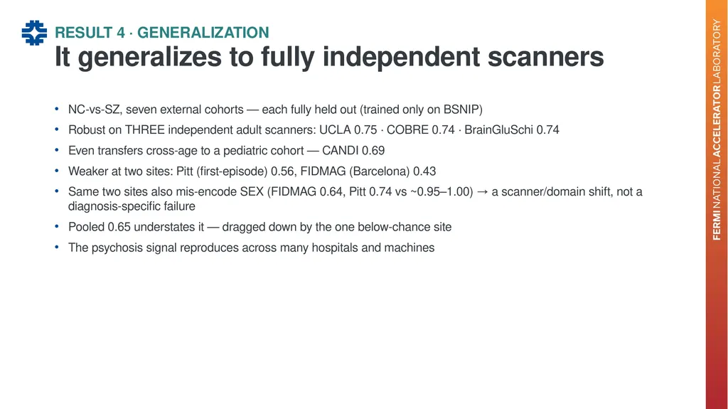
NC-vs-SZ, seven external cohorts — each fully held out (trained only on BSNIP)
Robust on THREE independent adult scanners: UCLA 0.75 · COBRE 0.74 · BrainGluSchi 0.74
Even transfers cross-age to a pediatric cohort — CANDI 0.69
Weaker at two sites: Pitt (first-episode) 0.56, FIDMAG (Barcelona) 0.43
Same two sites also mis-encode SEX (FIDMAG 0.64, Pitt 0.74 vs ~0.95–1.00) → a scanner/domain shift, not a diagnosis-specific failure
Pooled 0.65 understates it — dragged down by the one below-chance site
The psychosis signal reproduces across many hospitals and machines It generalizes to fully independent scanners RESULT 4 · GENERALIZATION<br>

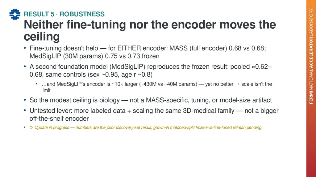
Fine-tuning doesn't help — for EITHER encoder: MASS (full encoder) 0.68 vs 0.68; MedSigLIP (30M params) 0.75 vs 0.73 frozen
A second foundation model (MedSigLIP) reproduces the frozen result: pooled ≈0.62–0.68, same controls (sex ~0.95, age r ~0.8)
…and MedSigLIP's encoder is ~10× larger (≈430M vs ≈40M params) — yet no better → scale isn't the limit
So the modest ceiling is biology — not a MASS-specific, tuning, or model-size artifact
Untested lever: more labeled data + scaling the same 3D-medical family — not a bigger off-the-shelf encoder
⟳ Update in progress — numbers are the prior discovery-set result; grown-N matched-split frozen-vs-fine-tuned refresh pending. Neither fine-tuning nor the encoder moves the ceiling RESULT 5 · ROBUSTNESS<br>

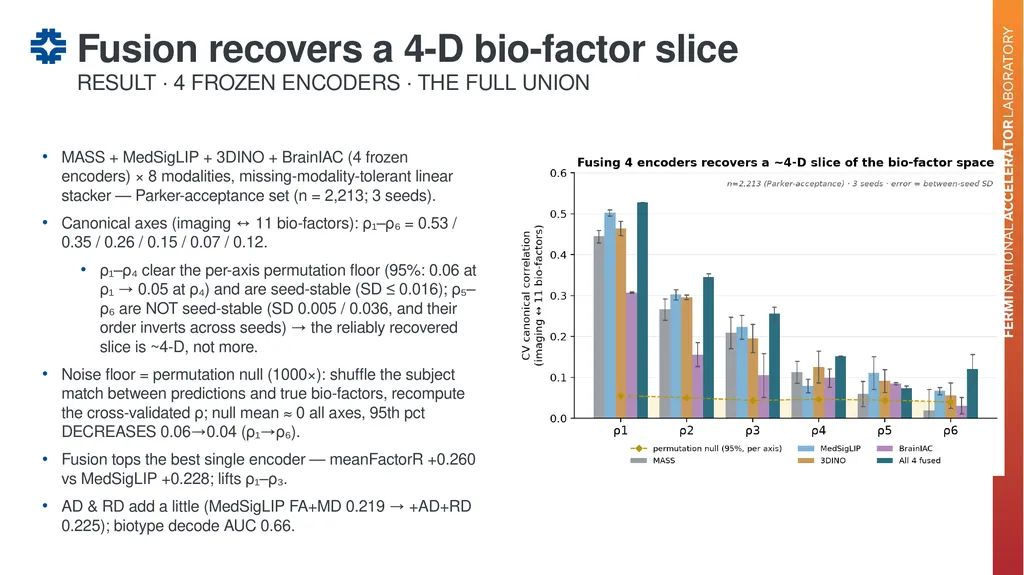
MASS + MedSigLIP + 3DINO + BrainIAC (4 frozen encoders) × 8 modalities, missing-modality-tolerant linear stacker — Parker-acceptance set (n = 2,213; 3 seeds).
Canonical axes (imaging ↔ 11 bio-factors): ρ₁–ρ₆ = 0.53 / 0.35 / 0.26 / 0.15 / 0.07 / 0.12.
ρ₁–ρ₄ clear the per-axis permutation floor (95%: 0.06 at ρ₁ → 0.05 at ρ₄) and are seed-stable (SD ≤ 0.016); ρ₅–ρ₆ are NOT seed-stable (SD 0.005 / 0.036, and their order inverts across seeds) → the reliably recovered slice is ~4-D, not more.
Noise floor = permutation null (1000×): shuffle the subject match between predictions and true bio-factors, recompute the cross-validated ρ; null mean ≈ 0 all axes, 95th pct DECREASES 0.06→0.04 (ρ₁→ρ₆).
Fusion tops the best single encoder — meanFactorR +0.260 vs MedSigLIP +0.228; lifts ρ₁–ρ₃.
AD & RD add a little (MedSigLIP FA+MD 0.219 → +AD+RD 0.225); biotype decode AUC 0.66. Fusion recovers a 4-D bio-factor slice RESULT · 4 FROZEN ENCODERS · THE FULL UNION<br>

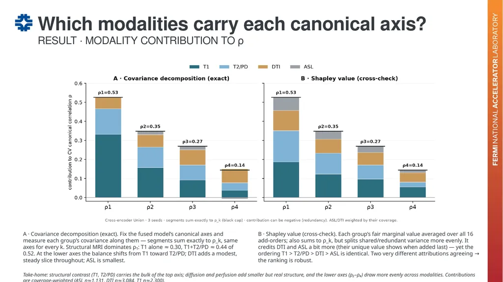
Which modalities carry each canonical axis? RESULT · MODALITY CONTRIBUTION TO ρ A · Covariance decomposition (exact). Fix the fused model’s canonical axes and measure each group’s covariance along them — segments sum exactly to ρ_k, same axes for every k. Structural MRI dominates ρ₁: T1 alone ≈ 0.30, T1+T2/PD ≈ 0.44 of 0.52. At the lower axes the balance shifts from T1 toward T2/PD; DTI adds a modest, steady slice throughout; ASL is smallest. B · Shapley value (cross-check). Each group’s fair marginal value averaged over all 16 add-orders; also sums to ρ_k, but splits shared/redundant variance more evenly. It credits DTI and ASL a bit more (their unique value shows when added last) — yet the ordering T1 > T2/PD > DTI > ASL is identical. Two very different attributions agreeing → the ranking is robust. Take-home: structural contrast (T1, T2/PD) carries the bulk of the top axis; diffusion and perfusion add smaller but real structure, and the lower axes (ρ₂–ρ₄) draw more evenly across modalities. Contributions are coverage-weighted (ASL n≈1,131, DTI n≈3,084, T1 n≈2,300).<br>

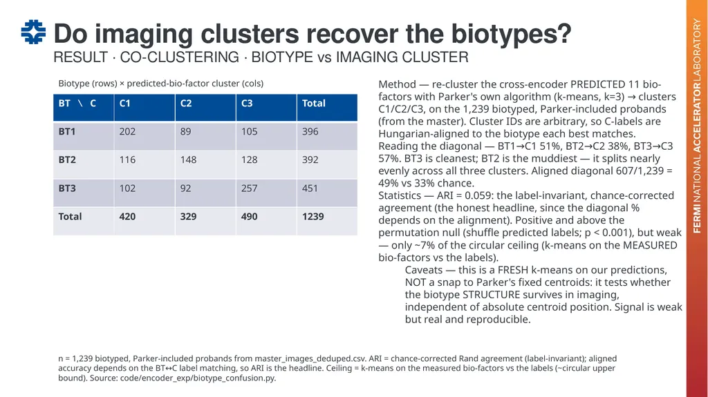
RESULT · CO-CLUSTERING · BIOTYPE vs IMAGING CLUSTER Do imaging clusters recover the biotypes? n = 1,239 biotyped, Parker-included probands from master_images_deduped.csv. ARI = chance-corrected Rand agreement (label-invariant); aligned accuracy depends on the BT↔C label matching, so ARI is the headline. Ceiling = k-means on the measured bio-factors vs the labels (~circular upper bound). Source: code/encoder_exp/biotype_confusion.py. Biotype (rows) × predicted-bio-factor cluster (cols) Method — re-cluster the cross-encoder PREDICTED 11 bio-factors with Parker's own algorithm (k-means, k=3) → clusters C1/C2/C3, on the 1,239 biotyped, Parker-included probands (from the master). Cluster IDs are arbitrary, so C-labels are Hungarian-aligned to the biotype each best matches.
Reading the diagonal — BT1→C1 51%, BT2→C2 38%, BT3→C3 57%. BT3 is cleanest; BT2 is the muddiest — it splits nearly evenly across all three clusters. Aligned diagonal 607/1,239 = 49% vs 33% chance.
Statistics — ARI = 0.059: the label-invariant, chance-corrected agreement (the honest headline, since the diagonal % depends on the alignment). Positive and above the permutation null (shuffle predicted labels; p < 0.001), but weak — only ~7% of the circular ceiling (k-means on the MEASURED bio-factors vs the labels).
Caveats — this is a FRESH k-means on our predictions, NOT a snap to Parker's fixed centroids: it tests whether the biotype STRUCTURE survives in imaging, independent of absolute centroid position. Signal is weak but real and reproducible.<br>

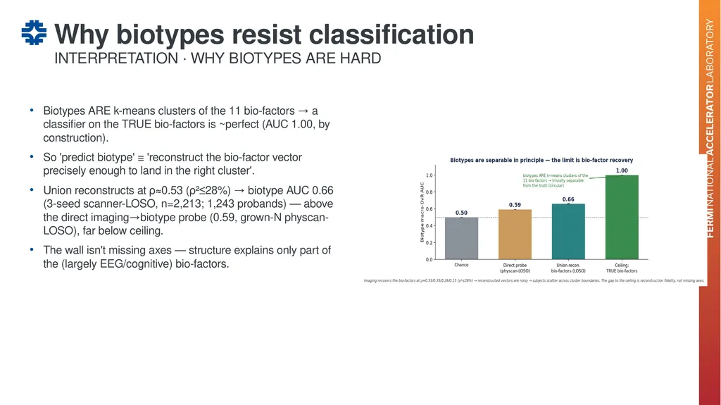
Biotypes ARE k-means clusters of the 11 bio-factors → a classifier on the TRUE bio-factors is ~perfect (AUC 1.00, by construction).
So 'predict biotype' ≡ 'reconstruct the bio-factor vector precisely enough to land in the right cluster'.
Union reconstructs at ρ≈0.53 (ρ²≤28%) → biotype AUC 0.66 (3-seed scanner-LOSO, n=2,213; 1,243 probands) — above the direct imaging→biotype probe (0.59, grown-N physcan-LOSO), far below ceiling.
The wall isn't missing axes — structure explains only part of the (largely EEG/cognitive) bio-factors. Why biotypes resist classification INTERPRETATION · WHY BIOTYPES ARE HARD<br>

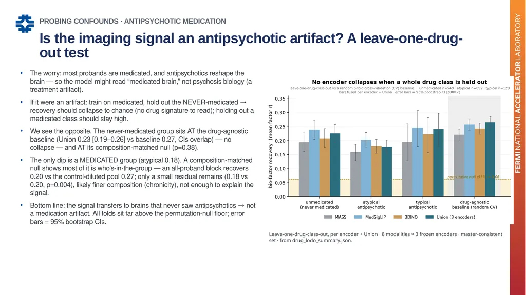
The worry: most probands are medicated, and antipsychotics reshape the brain — so the model might read “medicated brain,” not psychosis biology (a treatment artifact).
If it were an artifact: train on medicated, hold out the NEVER-medicated → recovery should collapse to chance (no drug signature to read); holding out a medicated class should stay high.
We see the opposite. The never-medicated group sits AT the drug-agnostic baseline (Union 0.23 [0.19–0.26] vs baseline 0.27, CIs overlap) — no collapse — and AT its composition-matched null (p=0.38).
The only dip is a MEDICATED group (atypical 0.18). A composition-matched null shows most of it is who’s-in-the-group — an all-proband block recovers 0.20 vs the control-diluted pool 0.27; only a small residual remains (0.18 vs 0.20, p=0.004), likely finer composition (chronicity), not enough to explain the signal.
Bottom line: the signal transfers to brains that never saw antipsychotics → not a medication artifact. All folds sit far above the permutation-null floor; error bars = 95% bootstrap CIs. Is the imaging signal an antipsychotic artifact? A leave-one-drug-out test PROBING CONFOUNDS · ANTIPSYCHOTIC MEDICATION Leave-one-drug-class-out, per encoder + Union · 8 modalities × 3 frozen encoders · master-consistent set · from drug_lodo_summary.json.<br>

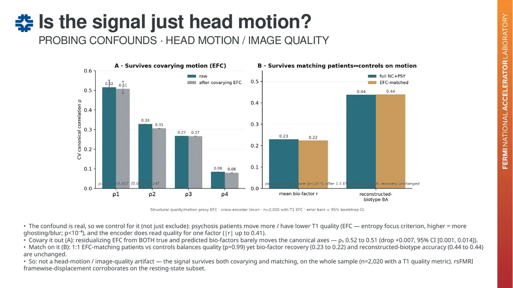
Is the signal just head motion? PROBING CONFOUNDS · HEAD MOTION / IMAGE QUALITY • The confound is real, so we control for it (not just exclude): psychosis patients move more / have lower T1 quality (EFC — entropy focus criterion, higher = more ghosting/blur; p<10⁻⁴), and the encoder does read quality for one factor (|r| up to 0.41).
• Covary it out (A): residualizing EFC from BOTH true and predicted bio-factors barely moves the canonical axes — ρ₁ 0.52 to 0.51 (drop +0.007, 95% CI [0.001, 0.014]).
• Match on it (B): 1:1 EFC-matching patients vs controls balances quality (p=0.99) yet bio-factor recovery (0.23 to 0.22) and reconstructed-biotype accuracy (0.44 to 0.44) are unchanged.
• So: not a head-motion / image-quality artifact — the signal survives both covarying and matching, on the whole sample (n=2,020 with a T1 quality metric). rsFMRI framewise-displacement corroborates on the resting-state subset.<br>

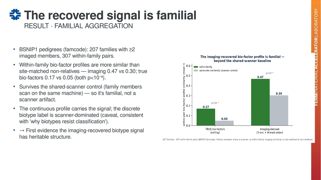
BSNIP1 pedigrees (famcode): 207 families with ≥2 imaged members, 307 within-family pairs.
Within-family bio-factor profiles are more similar than site-matched non-relatives — imaging 0.47 vs 0.30; true bio-factors 0.17 vs 0.05 (both p<10⁻⁴).
Survives the shared-scanner control (family members scan on the same machine) — so it's familial, not a scanner artifact.
The continuous profile carries the signal; the discrete biotype label is scanner-dominated (caveat, consistent with 'why biotypes resist classification').
→ First evidence the imaging-recovered biotype signal has heritable structure. The recovered signal is familial RESULT · FAMILIAL AGGREGATION<br>

Where this goes 04<br>

Take-home: a real, generalizable brain signal exists — small for DSM categories, strongest as dimensional bio-factors (ρ₁ ≈ 0.52; a ~4-D recovered slice — ρ₁–ρ₄ clear the permutation noise floor across 5 seeds, ρ₅ sits at it) and biotypes over DSM.
Already done (was on this roadmap): all 8 modalities × 3 frozen encoders fused on n = 2,230 — T1 · T2/PD · 4×DTI · ASL; diffusion & perfusion add only a little.
The signal is weak but not zero — pulled out of the union of diverse frozen models. Model size is not currently a factor: a ~10× larger encoder (MedSigLIP) and fine-tuning don't help.
Extract more by: more labeled data · dimensional (bio-factor) targets · purpose-built 3D-medical pretraining scaled up.
Compute: heavy training → UChicago Midway3 (A100 GPUs). Weak but real → scale the signal INTERPRETATION & ROADMAP<br>

Biotype bio-factor data — the eleven bio-factors (Parker et al. 2026); we now have all three cohorts
Additional modalities with shared IDs — DTI (white matter) & ASL (perfusion), to test if they separate Biotype axes (Pattern-1 vs Pattern-2)
Access help for the COBRE, FBIRN and MPRC external cohorts
Feedback on the clinical framing for the manuscript (AJP draft in progress) What we need next HOW THE COLLABORATION CAN HELP<br>

Thank you — questions welcome
A real, generalizable brain signal for psychosis exists: small for DSM categories, stronger for biology-based biotypes and cognition — and it is ours to scale.
BSNIP / PARDIP Collaboration · MASS encoder (Stanford-AIMI)<br>

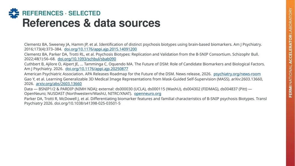
References & data sources REFERENCES · SELECTED Clementz BA, Sweeney JA, Hamm JP, et al. Identification of distinct psychosis biotypes using brain-based biomarkers. Am J Psychiatry. 2016;173(4):373–384. doi.org/10.1176/appi.ajp.2015.14091200
Clementz BA, Parker DA, Trotti RL, et al. Psychosis Biotypes: Replication and Validation from the B-SNIP Consortium. Schizophr Bull. 2022;48(1):56–68. doi.org/10.1093/schbul/sbab090
Cuthbert B, Ajilore O, Alpert JE, … Tamminga C, Oquendo MA. The Future of DSM: Role of Candidate Biomarkers and Biological Factors. Am J Psychiatry. 2026. doi.org/10.1176/appi.ajp.20250877
American Psychiatric Association. APA Releases Roadmap for the Future of the DSM. News release, 2026. psychiatry.org/news-room
Gao Y, et al. Learning Generalizable 3D Medical Image Representations from Mask-Guided Self-Supervision (MASS). arXiv:2603.13660, 2026. arxiv.org/abs/2603.13660
Data — BSNIP1/2 & PARDIP (NIMH NDA); external: ds000030 (UCLA), ds000115 (WashU), ds004302 (FIDMAG), ds004837 (Pitt) — OpenNeuro; NUSDAST (Northwestern/WashU, NITRC/XNAT). openneuro.org
Parker DA, Trotti R, McDowell J, et al. Differentiating biomarker features and familial characteristics of B-SNIP psychosis Biotypes. Transl Psychiatry 2026. doi.org/10.1038/s41398-025-03501-5<br>

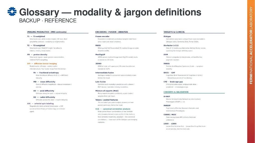
Glossary — modality & jargon definitions BACKUP · REFERENCE<br>

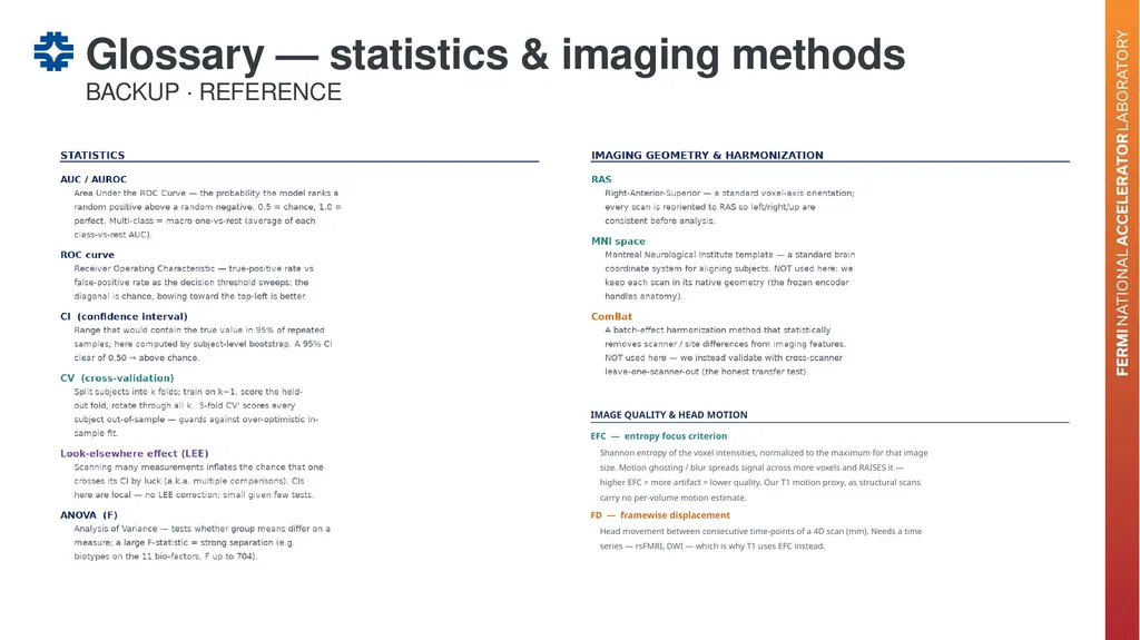
Glossary — statistics & imaging methods BACKUP · REFERENCE IMAGE QUALITY & HEAD MOTION
EFC — entropy focus criterion
Shannon entropy of the voxel intensities, normalized to the maximum for that image size. Motion ghosting / blur spreads signal across more voxels and RAISES it — higher EFC = more artifact = lower quality. Our T1 motion proxy, as structural scans carry no per-volume motion estimate.
FD — framewise displacement
Head movement between consecutive time-points of a 4D scan (mm). Needs a time series — rsFMRI, DWI — which is why T1 uses EFC instead.<br>

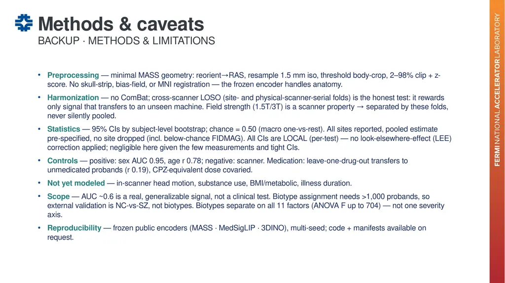
Preprocessing — minimal MASS geometry: reorient→RAS, resample 1.5 mm iso, threshold body-crop, 2–98% clip + z-score. No skull-strip, bias-field, or MNI registration — the frozen encoder handles anatomy.
Harmonization — no ComBat; cross-scanner LOSO (site- and physical-scanner-serial folds) is the honest test: it rewards only signal that transfers to an unseen machine. Field strength (1.5T/3T) is a scanner property → separated by these folds, never silently pooled.
Statistics — 95% CIs by subject-level bootstrap; chance = 0.50 (macro one-vs-rest). All sites reported, pooled estimate pre-specified, no site dropped (incl. below-chance FIDMAG). All CIs are LOCAL (per-test) — no look-elsewhere-effect (LEE) correction applied; negligible here given the few measurements and tight CIs.
Controls — positive: sex AUC 0.95, age r 0.78; negative: scanner. Medication: leave-one-drug-out transfers to unmedicated probands (r 0.19), CPZ-equivalent dose covaried.
Not yet modeled — in-scanner head motion, substance use, BMI/metabolic, illness duration.
Scope — AUC ~0.6 is a real, generalizable signal, not a clinical test. Biotype assignment needs >1,000 probands, so external validation is NC-vs-SZ, not biotypes. Biotypes separate on all 11 factors (ANOVA F up to 704) — not one severity axis.
Reproducibility — frozen public encoders (MASS · MedSigLIP · 3DINO), multi-seed; code + manifests available on request. Methods & caveats BACKUP · METHODS & LIMITATIONS<br>

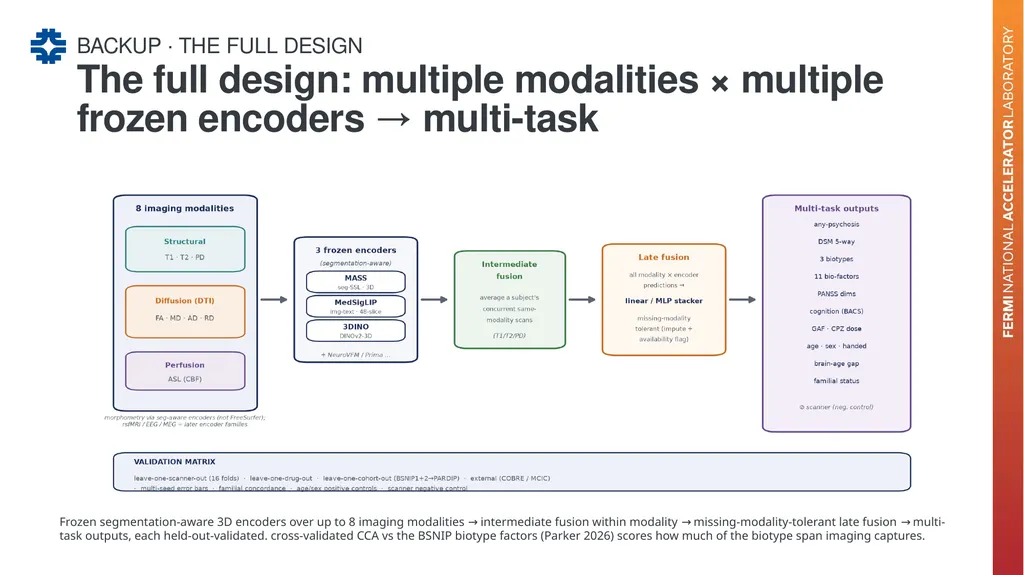
The full design: multiple modalities × multiple frozen encoders → multi-task BACKUP · THE FULL DESIGN Frozen segmentation-aware 3D encoders over up to 8 imaging modalities → intermediate fusion within modality → missing-modality-tolerant late fusion → multi-task outputs, each held-out-validated. cross-validated CCA vs the BSNIP biotype factors (Parker 2026) scores how much of the biotype span imaging captures.<br>

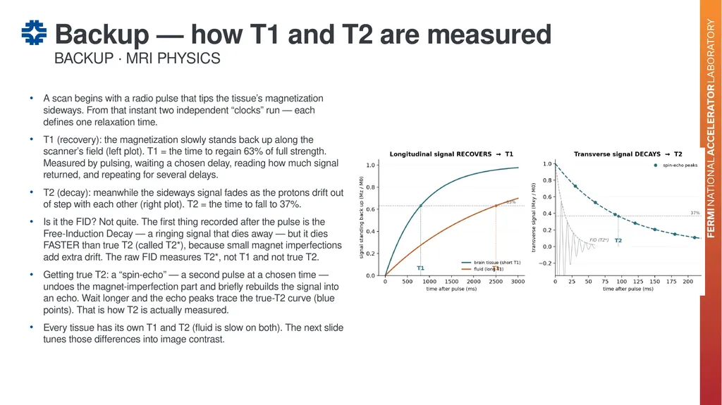
A scan begins with a radio pulse that tips the tissue’s magnetization sideways. From that instant two independent “clocks” run — each defines one relaxation time.
T1 (recovery): the magnetization slowly stands back up along the scanner’s field (left plot). T1 = the time to regain 63% of full strength. Measured by pulsing, waiting a chosen delay, reading how much signal returned, and repeating for several delays.
T2 (decay): meanwhile the sideways signal fades as the protons drift out of step with each other (right plot). T2 = the time to fall to 37%.
Is it the FID? Not quite. The first thing recorded after the pulse is the Free-Induction Decay — a ringing signal that dies away — but it dies FASTER than true T2 (called T2*), because small magnet imperfections add extra drift. The raw FID measures T2*, not T1 and not true T2.
Getting true T2: a “spin-echo” — a second pulse at a chosen time — undoes the magnet-imperfection part and briefly rebuilds the signal into an echo. Wait longer and the echo peaks trace the true-T2 curve (blue points). That is how T2 is actually measured.
Every tissue has its own T1 and T2 (fluid is slow on both). The next slide tunes those differences into image contrast. Backup — how T1 and T2 are measured BACKUP · MRI PHYSICS<br>

MRI contrast comes from how a tissue responds to a radio pulse. Two tissue properties drive it:
T1 — how fast the signal “resets” between pulses (recovery). T2 — how fast the signal fades after each pulse (decay). Fat, brain tissue, and water each have their own T1 and T2 — that is what makes them look different.
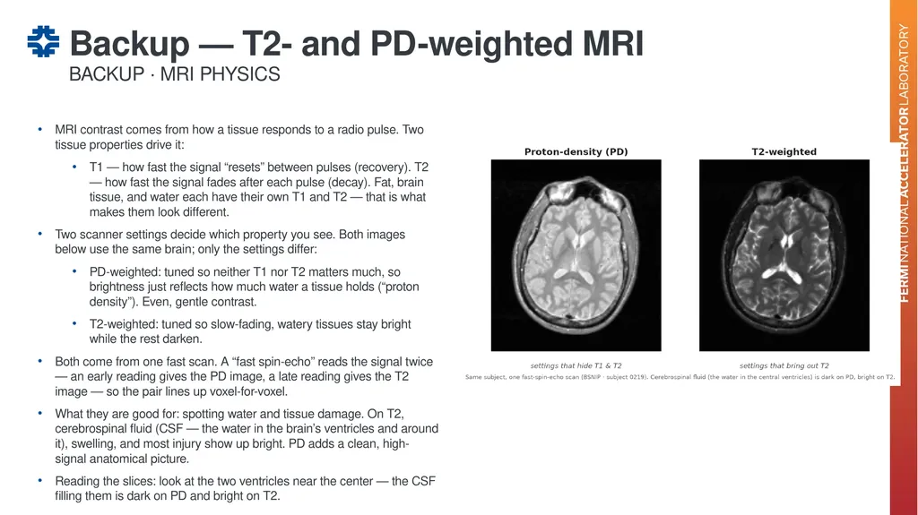
Two scanner settings decide which property you see. Both images below use the same brain; only the settings differ:
PD-weighted: tuned so neither T1 nor T2 matters much, so brightness just reflects how much water a tissue holds (“proton density”). Even, gentle contrast.
T2-weighted: tuned so slow-fading, watery tissues stay bright while the rest darken.
Both come from one fast scan. A “fast spin-echo” reads the signal twice — an early reading gives the PD image, a late reading gives the T2 image — so the pair lines up voxel-for-voxel.
What they are good for: spotting water and tissue damage. On T2, cerebrospinal fluid (CSF — the water in the brain’s ventricles and around it), swelling, and most injury show up bright. PD adds a clean, high-signal anatomical picture.
Reading the slices: look at the two ventricles near the center — the CSF filling them is dark on PD and bright on T2. Backup — T2- and PD-weighted MRI BACKUP · MRI PHYSICS<br>

DTI watches how water molecules drift (diffuse) inside the brain. The scan is sensitised to motion along many directions, so each voxel reports not just how much water moves but which way.
In a fibre bundle, water slides easily ALONG the axons but is blocked ACROSS them. Fitting this directional pattern gives, per voxel, a small ellipsoid (a “tensor”) — long where diffusion is directional, round where it is free.
Four numbers summarise that ellipsoid — the maps at right (all from ONE scan):
FA — fractional anisotropy: how directional the diffusion is (0 = free, 1 = strongly aligned). White-matter tracts are bright; grey matter is dark.
MD — mean diffusivity: overall water mobility, averaged over directions.
AD — axial diffusivity: mobility along the fibre; RD — radial diffusivity: mobility across it. AD vs RD helps separate fibre integrity from the myelin sheath around it.
Why we use it: white-matter organisation is disrupted in psychosis, so these maps add tissue microstructure that T1/T2/PD (which show anatomy, not fibre direction) cannot. Backup — diffusion tensor imaging (DTI) BACKUP · MRI PHYSICS<br>

ASL (arterial spin labeling) maps cerebral blood flow — how much blood each bit of brain tissue receives — with NO injected dye. The blood itself is the tracer.
How it works: a radio pulse magnetically “tags” the water in arterial blood in the neck; after a short wait the tagged blood flows up into the brain, and you image. Subtract from an untagged image — what remains is the signal carried IN by blood → a blood-flow map.
The signal is tiny (~1% of the brain signal), so many tag/image pairs are averaged. That makes ASL noisier and lower-resolution than the structural scans — and it was collected on fewer subjects (n≈1,131), which is why it contributes least on the previous slides.
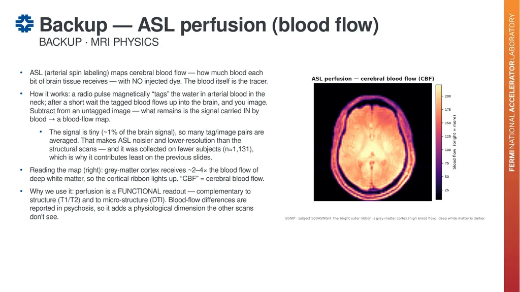
Reading the map (right): grey-matter cortex receives ~2–4× the blood flow of deep white matter, so the cortical ribbon lights up. “CBF” = cerebral blood flow.
Why we use it: perfusion is a FUNCTIONAL readout — complementary to structure (T1/T2) and to micro-structure (DTI). Blood-flow differences are reported in psychosis, so it adds a physiological dimension the other scans don’t see. Backup — ASL perfusion (blood flow) BACKUP · MRI PHYSICS<br>

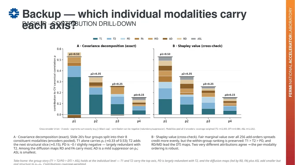
Backup — which individual modalities carry each axis? BACKUP · CONTRIBUTION DRILL-DOWN A · Covariance decomposition (exact). Slide 26’s four groups split into their 8 constituent modalities (encoders pooled). T1 alone carries ρ₁ (≈0.33 of 0.53); T2 adds the next structural slice (≈0.15). PD is ~0 / slightly negative — largely redundant with T2. Among the diffusion maps RD and FA carry most; AD is a mild suppressor on ρ₁; ASL is smallest. B · Shapley value (cross-check). Fair marginal value over all 256 add-orders spreads credit more evenly, but the within-group ranking is preserved: T1 > T2 > PD, and RD/MD lead the DTI maps. Two very different attributions agree → the per-modality ordering is robust. Take-home: the group story (T1 > T2/PD > DTI > ASL) holds at the individual level — T1 and T2 carry the top axis, PD is largely redundant with T2, and the diffusion maps (led by RD, FA) plus ASL add smaller but real structure to ρ₂–ρ₄. Contributions coverage-weighted.<br>

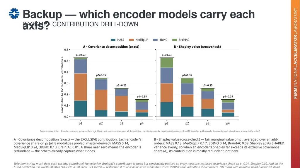
Backup — which encoder models carry each axis? BACKUP · CONTRIBUTION DRILL-DOWN A · Covariance decomposition (exact) — the EXCLUSIVE contribution. Each encoder’s covariance share on ρ₁ (all 8 modalities pooled, master-derived): MASS 0.14, MedSigLIP 0.24, 3DINO 0.13, BrainIAC 0.01. A share near zero means the encoder is redundant — the others already capture what it does. B · Shapley value (cross-check) — fair marginal value on ρ₁, averaged over all add-orders: MASS 0.13, MedSigLIP 0.17, 3DINO 0.14, BrainIAC 0.09. Shapley splits SHARED variance evenly, so when an encoder’s Shapley far exceeds its exclusive covariance share (A), its contribution is mostly redundant, not new. Take-home: How much does each encoder contribute? Not whether. BrainIAC's contribution is small but consistently positive on every measure: exclusive covariance share on ρ₁ 0.01, Shapley 0.09. And on the fused prediction it is worth +0.0070 (+0.2536 -> +0.2606, 3/3 seeds) — restricting it to only its positive modalities scores WORSE than admitting it everywhere, DTI maps with negative head r included. Read together: it is not a DISTINCT encoder — the incumbents already capture nearly all of what it sees — but it still buys variance reduction, which is why it helps the fusion without adding new signal. Under late fusion every model contributes something, however small (cf. Stein's example: combining even unrelated components lowers total risk), so the useful question is the SIZE of the contribution, not a pass/fail. (Canonical heads, 3 seeds; the incumbent 3 predate BrainIAC.)<br>

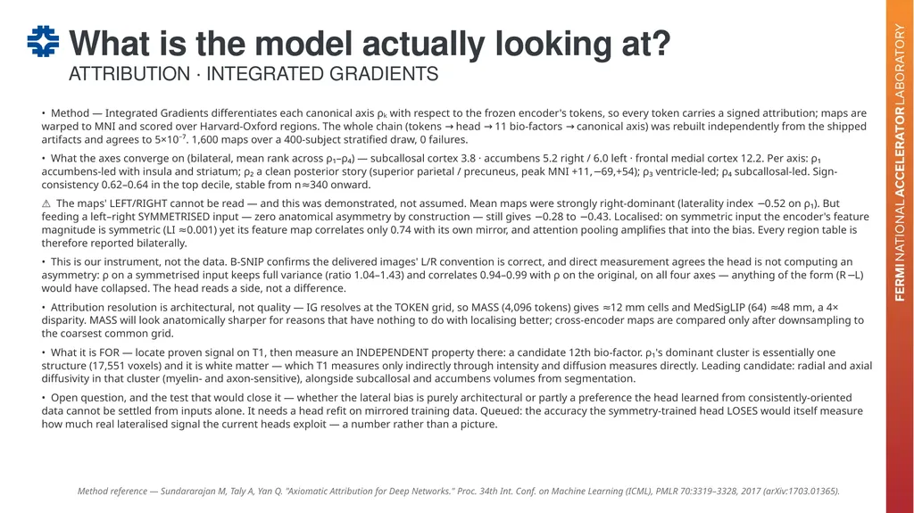
What is the model actually looking at? ATTRIBUTION · INTEGRATED GRADIENTS • Method — Integrated Gradients differentiates each canonical axis ρₖ with respect to the frozen encoder's tokens, so every token carries a signed attribution; maps are warped to MNI and scored over Harvard-Oxford regions. The whole chain (tokens → head → 11 bio-factors → canonical axis) was rebuilt independently from the shipped artifacts and agrees to 5×10⁻⁷. 1,600 maps over a 400-subject stratified draw, 0 failures.
• What the axes converge on (bilateral, mean rank across ρ₁–ρ₄) — subcallosal cortex 3.8 · accumbens 5.2 right / 6.0 left · frontal medial cortex 12.2. Per axis: ρ₁ accumbens-led with insula and striatum; ρ₂ a clean posterior story (superior parietal / precuneus, peak MNI +11,−69,+54); ρ₃ ventricle-led; ρ₄ subcallosal-led. Sign-consistency 0.62–0.64 in the top decile, stable from n≈340 onward.
⚠ The maps' LEFT/RIGHT cannot be read — and this was demonstrated, not assumed. Mean maps were strongly right-dominant (laterality index −0.52 on ρ₁). But feeding a left–right SYMMETRISED input — zero anatomical asymmetry by construction — still gives −0.28 to −0.43. Localised: on symmetric input the encoder's feature magnitude is symmetric (LI ≈0.001) yet its feature map correlates only 0.74 with its own mirror, and attention pooling amplifies that into the bias. Every region table is therefore reported bilaterally.
• This is our instrument, not the data. B-SNIP confirms the delivered images' L/R convention is correct, and direct measurement agrees the head is not computing an asymmetry: ρ on a symmetrised input keeps full variance (ratio 1.04–1.43) and correlates 0.94–0.99 with ρ on the original, on all four axes — anything of the form (R−L) would have collapsed. The head reads a side, not a difference.
• Attribution resolution is architectural, not quality — IG resolves at the TOKEN grid, so MASS (4,096 tokens) gives ≈12 mm cells and MedSigLIP (64) ≈48 mm, a 4× disparity. MASS will look anatomically sharper for reasons that have nothing to do with localising better; cross-encoder maps are compared only after downsampling to the coarsest common grid.
• What it is FOR — locate proven signal on T1, then measure an INDEPENDENT property there: a candidate 12th bio-factor. ρ₁'s dominant cluster is essentially one structure (17,551 voxels) and it is white matter — which T1 measures only indirectly through intensity and diffusion measures directly. Leading candidate: radial and axial diffusivity in that cluster (myelin- and axon-sensitive), alongside subcallosal and accumbens volumes from segmentation.
• Open question, and the test that would close it — whether the lateral bias is purely architectural or partly a preference the head learned from consistently-oriented data cannot be settled from inputs alone. It needs a head refit on mirrored training data. Queued: the accuracy the symmetry-trained head LOSES would itself measure how much real lateralised signal the current heads exploit — a number rather than a picture. Method reference — Sundararajan M, Taly A, Yan Q. "Axiomatic Attribution for Deep Networks." Proc. 34th Int. Conf. on Machine Learning (ICML), PMLR 70:3319–3328, 2017 (arXiv:1703.01365).<br>

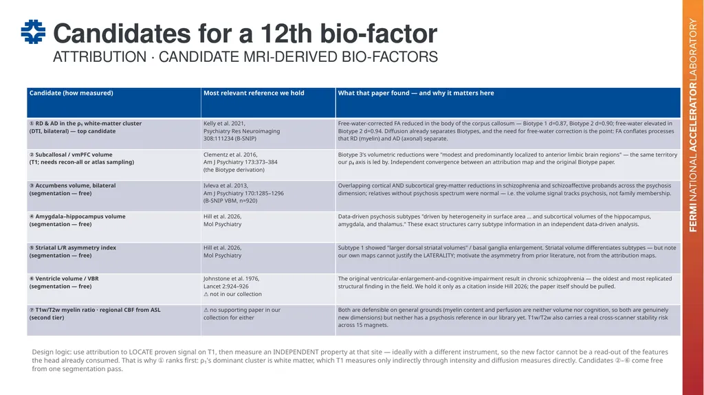
Candidates for a 12th bio-factor ATTRIBUTION · CANDIDATE MRI-DERIVED BIO-FACTORS Design logic: use attribution to LOCATE proven signal on T1, then measure an INDEPENDENT property at that site — ideally with a different instrument, so the new factor cannot be a read-out of the features the head already consumed. That is why ① ranks first: ρ₁'s dominant cluster is white matter, which T1 measures only indirectly through intensity and diffusion measures directly. Candidates ②–⑥ come free from one segmentation pass.<br>