Chapter 10. Potentials and fields 1 Chapter 10. Scalar and vector potentials where V is the new scalar potential 2 Scalar and vector potentials Note that the definitions of the potentials automatically take care of nonames and Faradays
"Chapter 10. Potentials and fields 1 Chapter 10." is the property of its rightful owner. Permission is granted to
download and print the materials on this website for personal, non-commercial use only, and to display it
on your personal computer provided you do not modify the materials and that you retain all copyright
notices contained in the materials. By downloading content from our website, you accept the terms of this
agreement.
Presentation Transcript
01
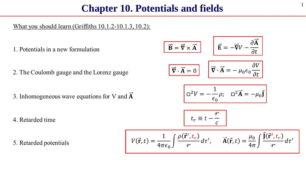
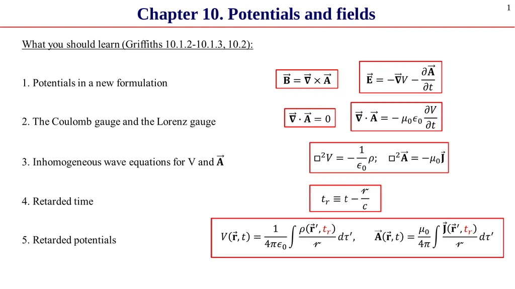
Chapter 10. Potentials and fields 1<br>
02
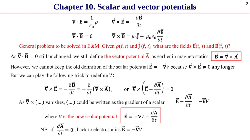
Chapter 10. Scalar and vector potentials where V is the new scalar potential 2<br>
03
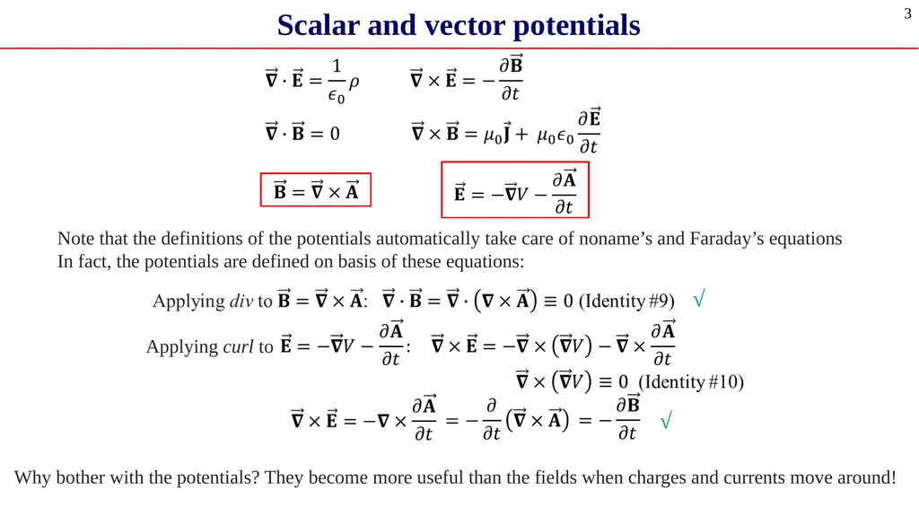
Scalar and vector potentials Note that the definitions of the potentials automatically take care of noname’s and Faraday’s equations In fact, the potentials are defined on basis of these equations: Applying curl to √ √ 3 Why bother with the potentials? They become more useful than the fields when charges and currents move around!<br>
04
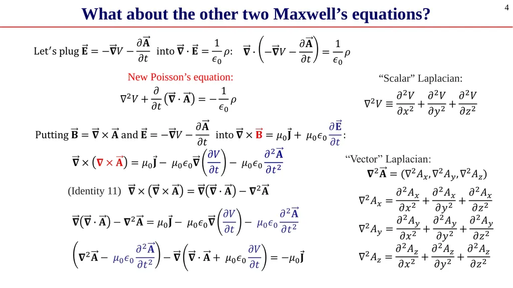
What about the other two Maxwell’s equations? New Poisson’s equation: “Scalar” Laplacian: (Identity 11) 4<br>
05
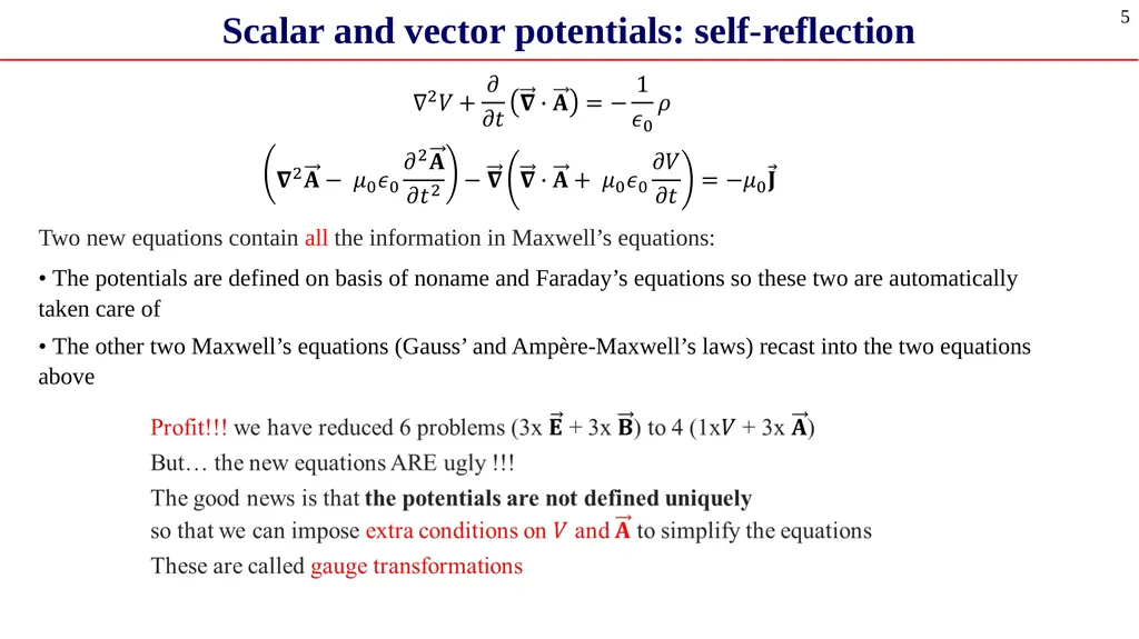
Scalar and vector potentials: self-reflection Two new equations contain all the information in Maxwell’s equations: 5 • The potentials are defined on basis of noname and Faraday’s equations so these two are automatically taken care of
• The other two Maxwell’s equations (Gauss’ and Ampère-Maxwell’s laws) recast into the two equations above<br>
06
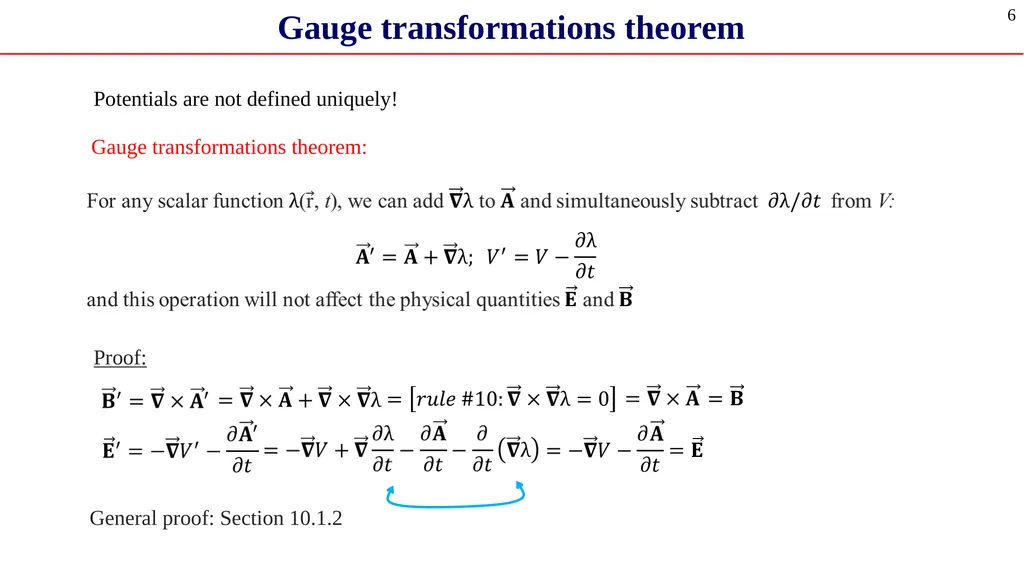
Gauge transformations theorem Proof: General proof: Section 10.1.2 6 Gauge transformations theorem: Potentials are not defined uniquely!<br>
07
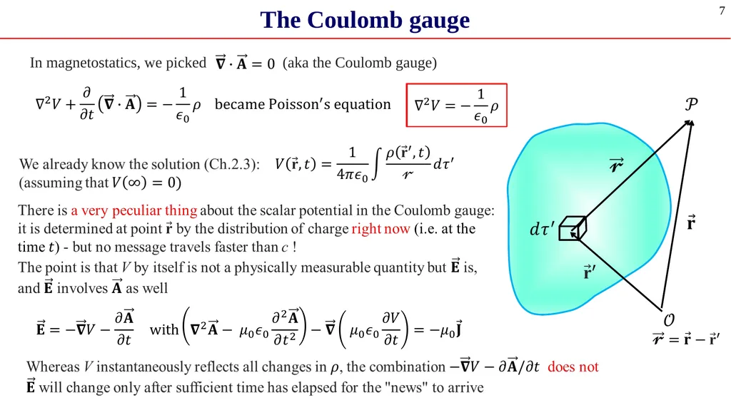
The Coulomb gauge In magnetostatics, we picked (aka the Coulomb gauge) 7<br>
08
The Lorenz gauge 8 Now we pick NB1: Not Dutch H.A. Lorentz, but Danish L.V. Lorenz
NB2: In case of the static scalar potential, Coulomb and Lorenz gauges become identical d'Alembertian operator: It’s called the Lorenz gauge Let’s do a bit of transformations over the equations for potentials So electrodynamics is reduced to solving these equations<br>
09
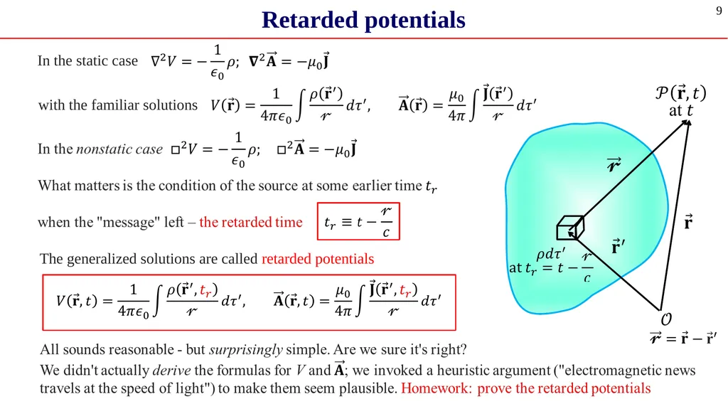
Retarded potentials In the static case with the familiar solutions The generalized solutions are called retarded potentials 9<br>
10
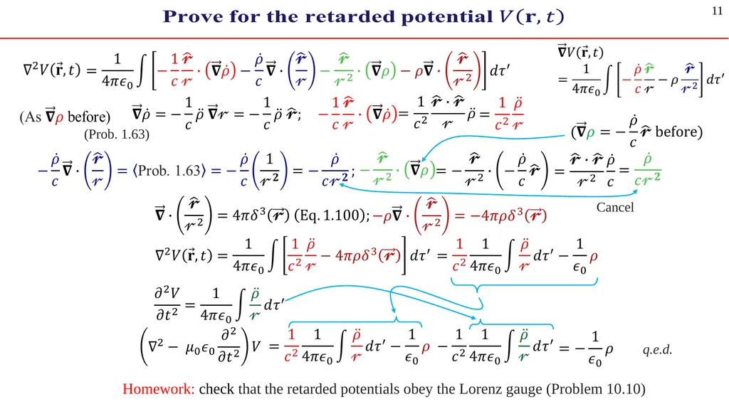
satisfies the inhomogeneous wave equation 10<br>
11
q.e.d. (Prob. 1.63) Cancel 11 Homework: check that the retarded potentials obey the Lorenz gauge (Problem 10.10)<br>
12
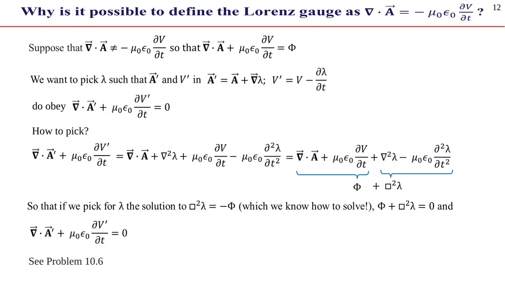
12 See Problem 10.6 do obey How to pick?<br>
13
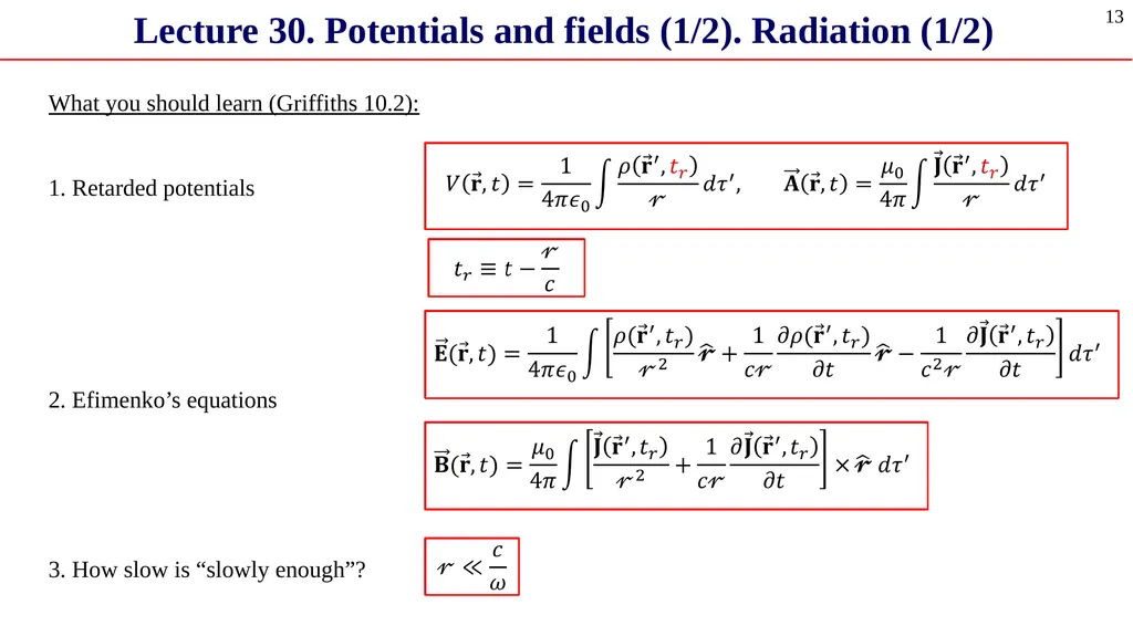
What you should learn (Griffiths 10.2):
1. Retarded potentials
2. Efimenko’s equations
3. How slow is “slowly enough”? Lecture 30. Potentials and fields (1/2). Radiation (1/2) 13<br>
14
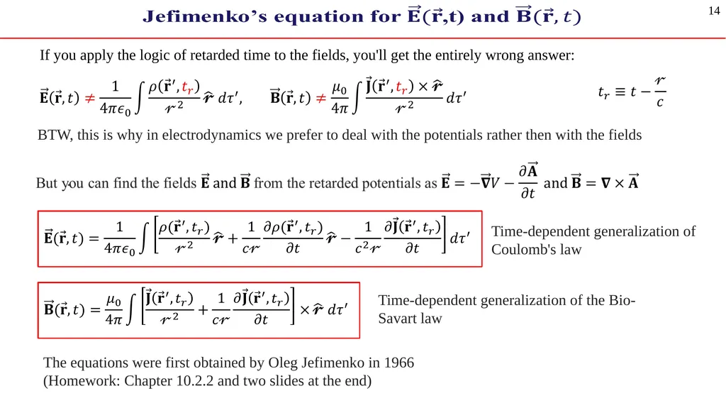
14 The equations were first obtained by Oleg Jefimenko in 1966
(Homework: Chapter 10.2.2 and two slides at the end) If you apply the logic of retarded time to the fields, you'll get the entirely wrong answer: BTW, this is why in electrodynamics we prefer to deal with the potentials rather then with the fields Time-dependent generalization of
Coulomb's law Time-dependent generalization of the Bio-Savart law<br>
15
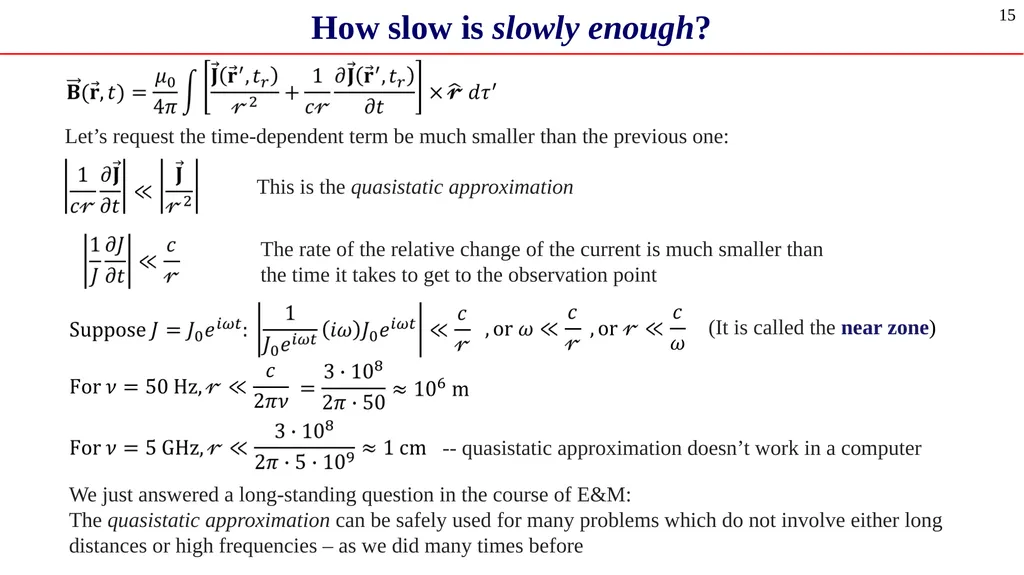
How slow is slowly enough? 15 (It is called the near zone) We just answered a long-standing question in the course of E&M:
The quasistatic approximation can be safely used for many problems which do not involve either long distances or high frequencies – as we did many times before Let’s request the time-dependent term be much smaller than the previous one: This is the quasistatic approximation -- quasistatic approximation doesn’t work in a computer The rate of the relative change of the current is much smaller than the time it takes to get to the observation point<br>
16
YouTube resources Youtube lectures by Jonathan Gardner: https://www.youtube.com/playlist?list=PLDDEED00333C1C30E
Scalar and vector potentials: https://www.youtube.com/watch?v=gc8NvnlMawY
Retarded potentials:
Part 1/3 https://www.youtube.com/watch?v=G4MdRbV-bgU
Part 3/3 https://www.youtube.com/watch?v=z9lC1rGLqDo&t=0s
Part 3/3 https://www.youtube.com/watch?v=0TXS9A6tjK4&t=49s 16<br>
17
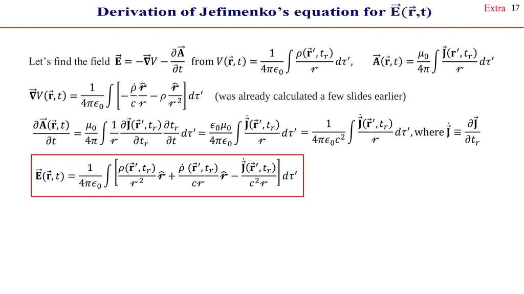
17 (was already calculated a few slides earlier)<br>
18
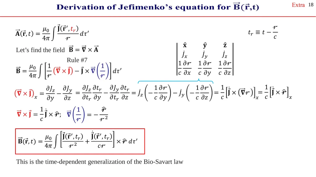
18 Let’s find the field This is the time-dependent generalization of the Bio-Savart law Rule #7<br>
19
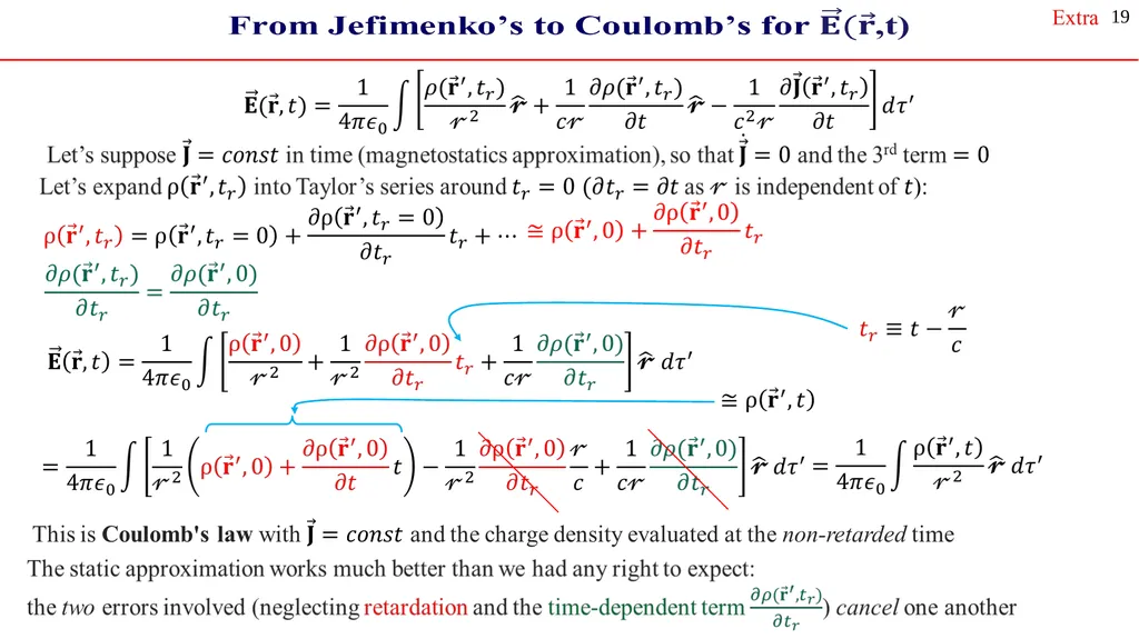
19<br>
20
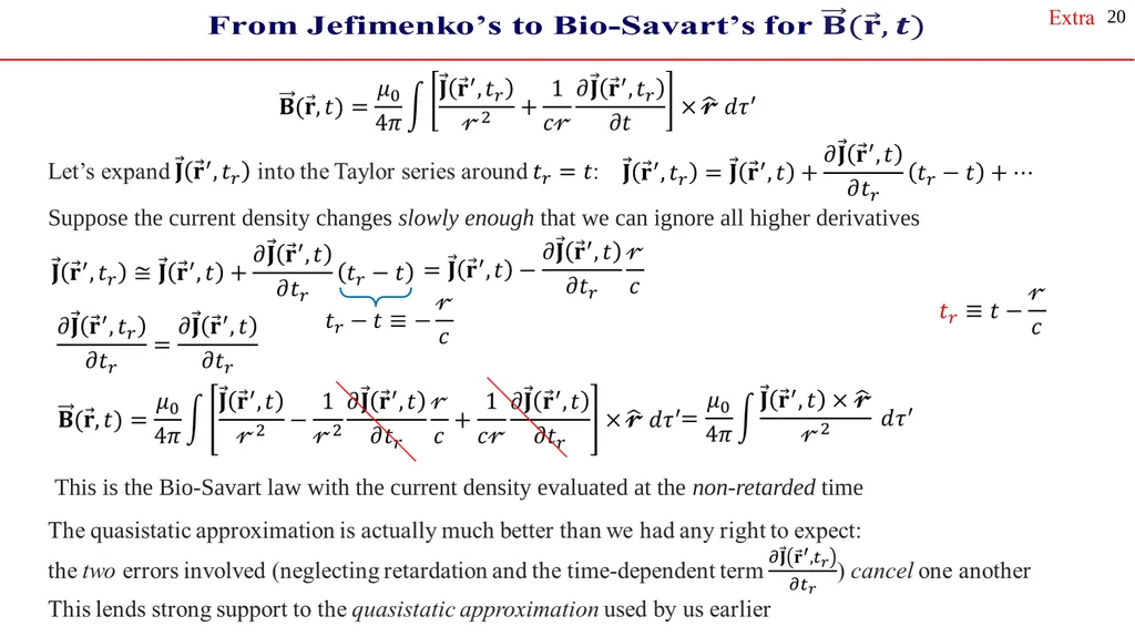
20 Suppose the current density changes slowly enough that we can ignore all higher derivatives This is the Bio-Savart law with the current density evaluated at the non-retarded time<br>
21
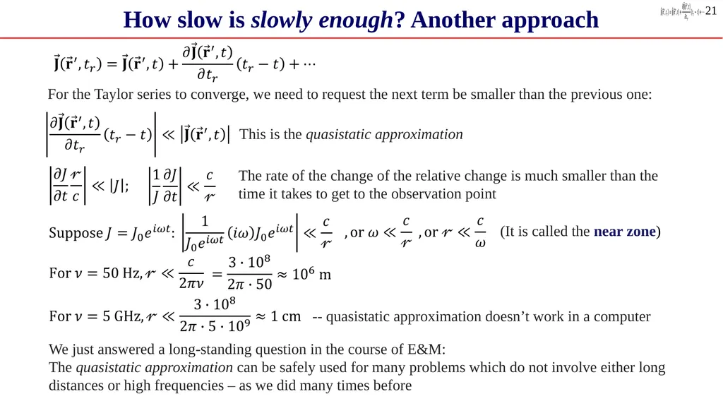
How slow is slowly enough? Another approach 21 (It is called the near zone) We just answered a long-standing question in the course of E&M:
The quasistatic approximation can be safely used for many problems which do not involve either long distances or high frequencies – as we did many times before For the Taylor series to converge, we need to request the next term be smaller than the previous one: This is the quasistatic approximation -- quasistatic approximation doesn’t work in a computer The rate of the change of the relative change is much smaller than the time it takes to get to the observation point<br>