
Chapter 14 Density Matrix State of a system at
Description: Chapter 14 Density Matrix State of a system at time t: Contains time dependent phase factors. Copyright Michael D. Fayer, 2018 Two state system: Copyright Michael D. Fayer, 2018 In general: ij density matrix element Copyright Michael
Related Topics
Download Presentation
"Chapter 14 Density Matrix State of a system at" is the property of its rightful owner. Permission is granted to download and print the materials on this website for personal, non-commercial use only, and to display it on your personal computer provided you do not modify the materials and that you retain all copyright notices contained in the materials. By downloading content from our website, you accept the terms of this agreement.
Presentation Transcript
slide1. Chapter 14<br>
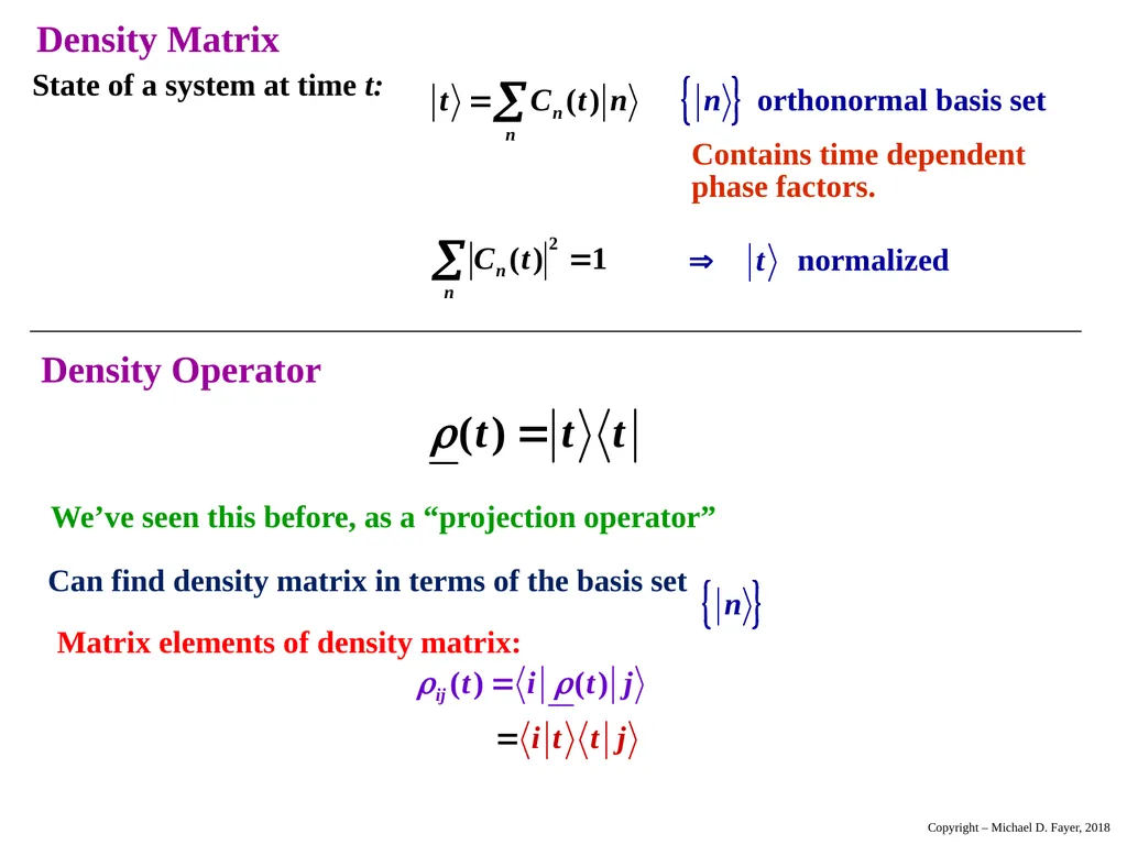
slide2. Density Matrix State of a system at time t: Contains time dependent
phase factors. Copyright – Michael D. Fayer, 2018<br>
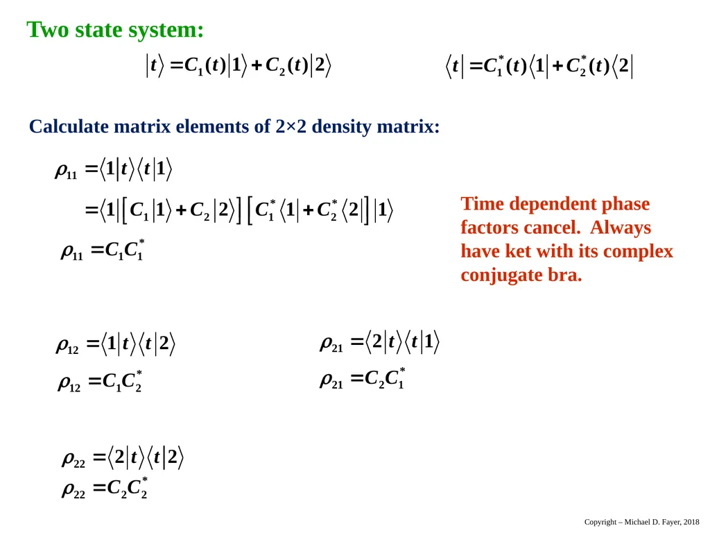
slide3. Two state system: Copyright – Michael D. Fayer, 2018<br>
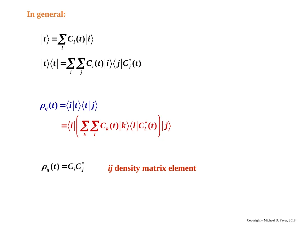
slide4. In general: ij density matrix element Copyright – Michael D. Fayer, 2018<br>
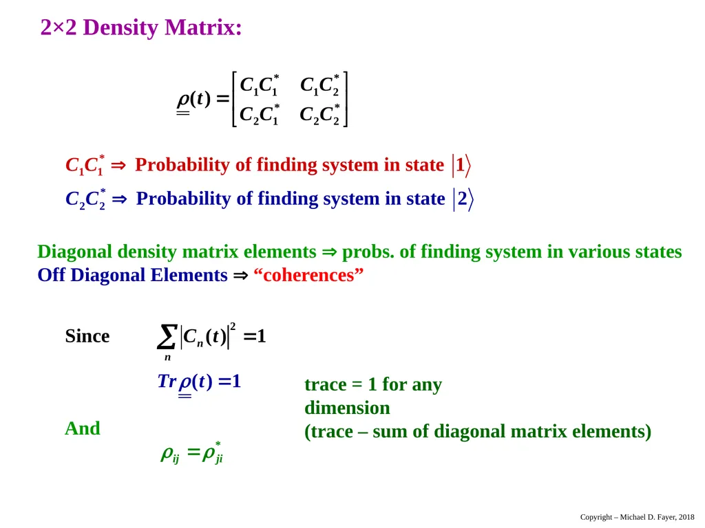
slide5. 2×2 Density Matrix: Diagonal density matrix elements probs. of finding system in various states
Off Diagonal Elements “coherences” Copyright – Michael D. Fayer, 2018<br>
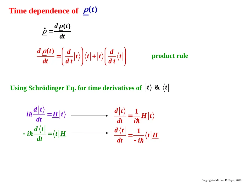
slide6. Time dependence of product rule Copyright – Michael D. Fayer, 2018<br>
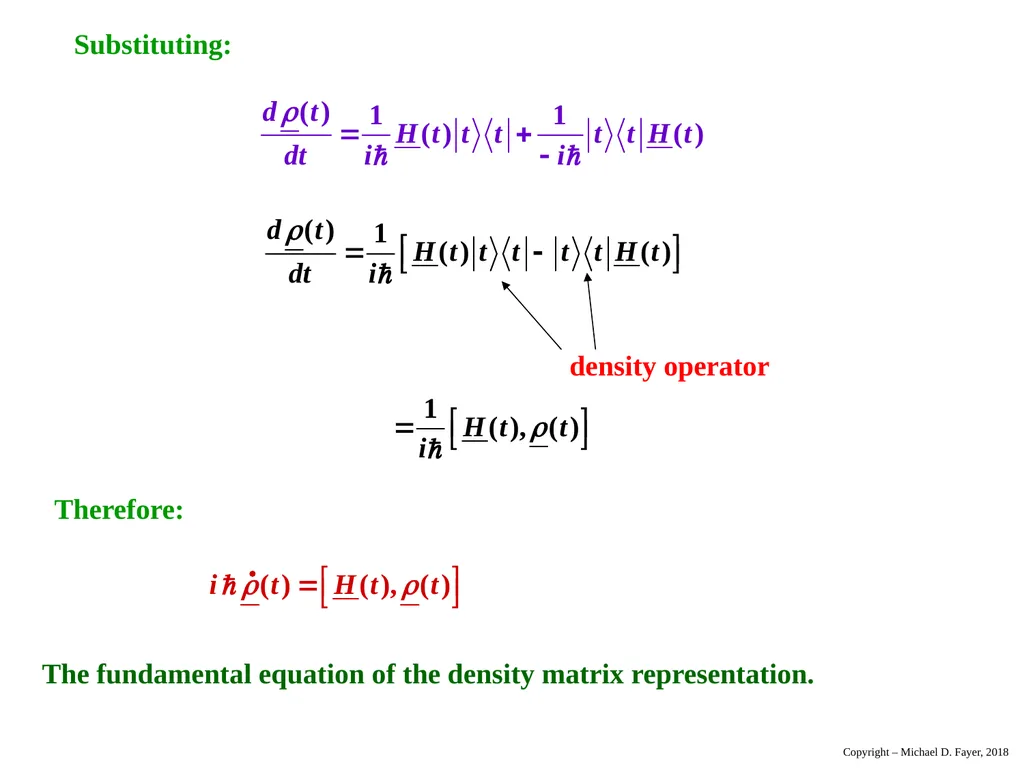
slide7. Substituting: density operator Copyright – Michael D. Fayer, 2018<br>
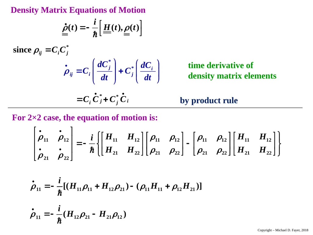
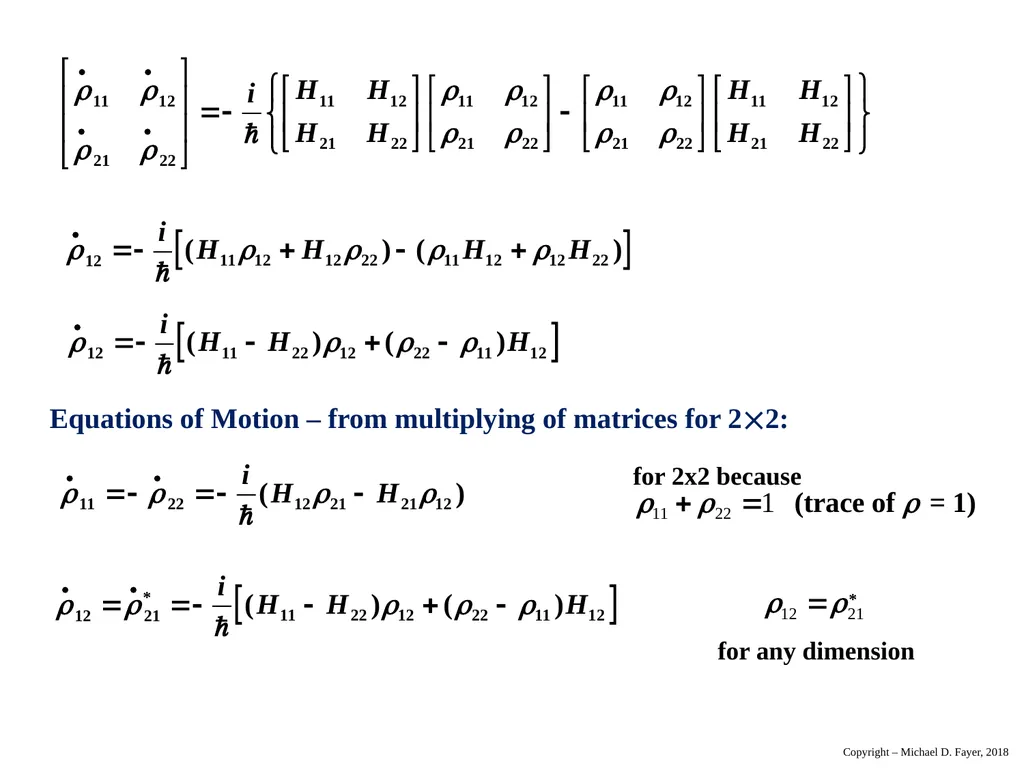
slide8. Density Matrix Equations of Motion by product rule time derivative of density matrix elements Copyright – Michael D. Fayer, 2018<br>
slide9. Copyright – Michael D. Fayer, 2018<br>
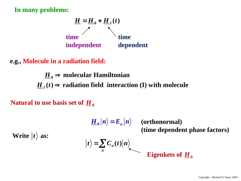
slide10. In many problems: time
independent time
dependent e.g., Molecule in a radiation field: Copyright – Michael D. Fayer, 2018<br>
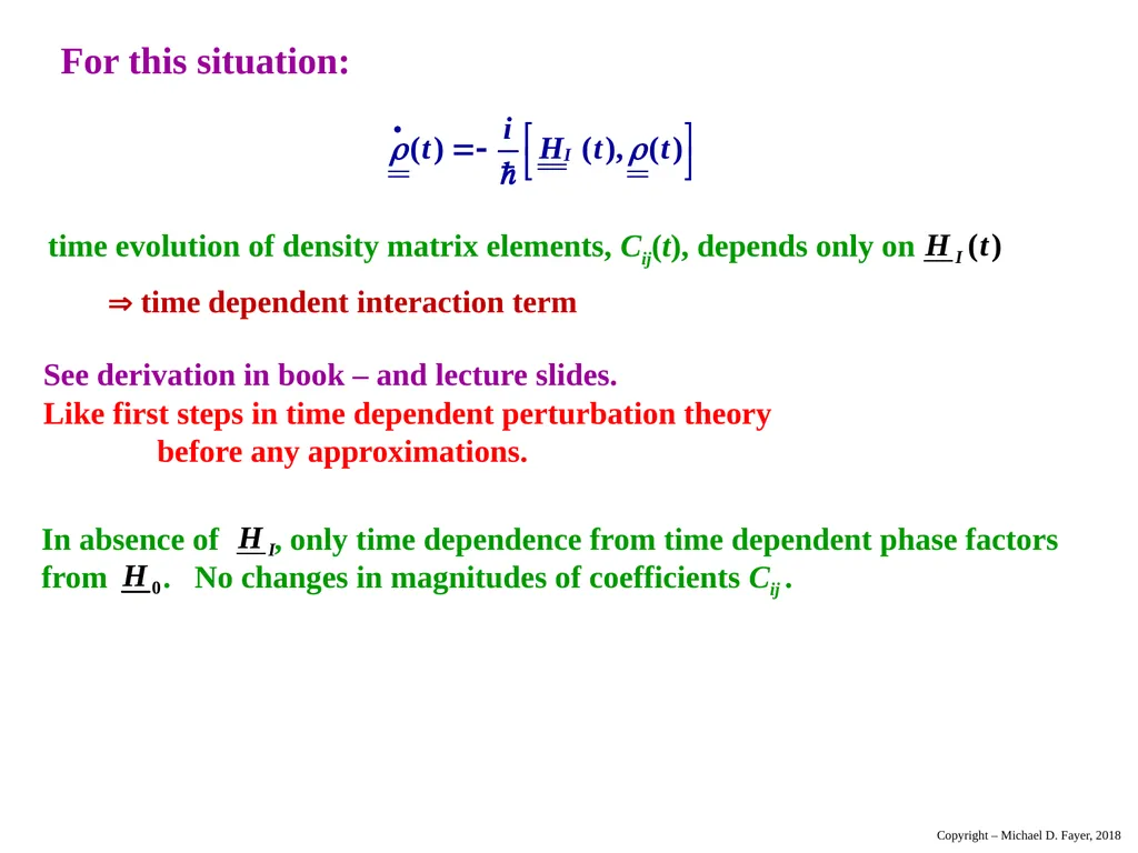
slide11. For this situation: time evolution of density matrix elements, Cij(t), depends only on time dependent interaction term See derivation in book – and lecture slides.
Like first steps in time dependent perturbation theory before any approximations. In absence of , only time dependence from time dependent phase factors
from . No changes in magnitudes of coefficients Cij . Copyright – Michael D. Fayer, 2018<br>
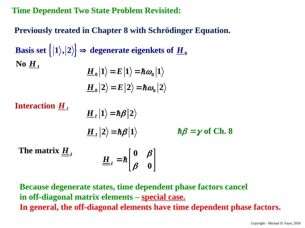
slide12. Time Dependent Two State Problem Revisited: Previously treated in Chapter 8 with Schrödinger Equation. Copyright – Michael D. Fayer, 2018<br>
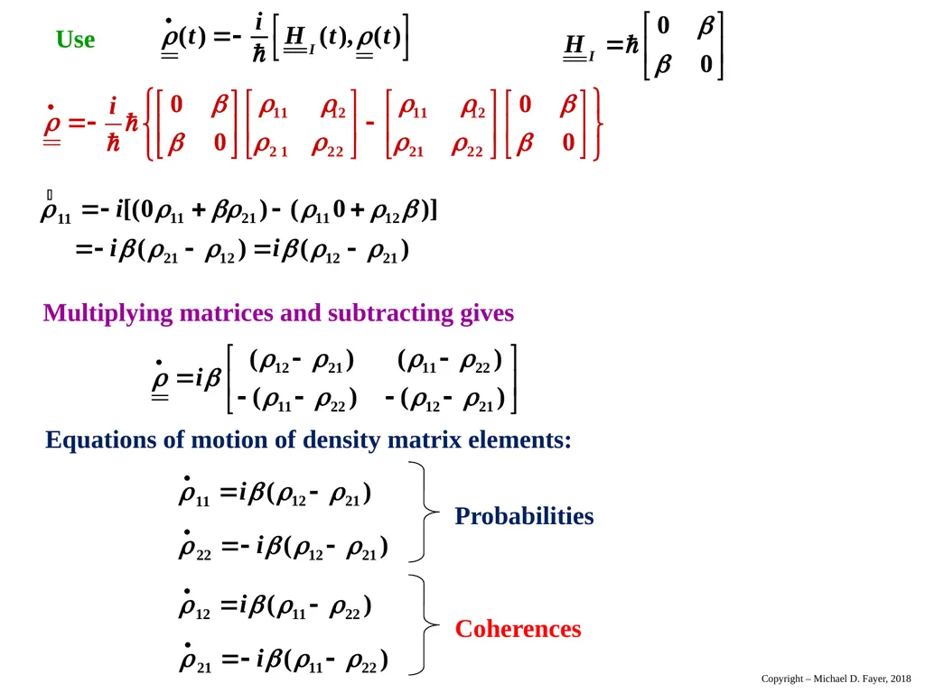
slide13. Use Copyright – Michael D. Fayer, 2018<br>
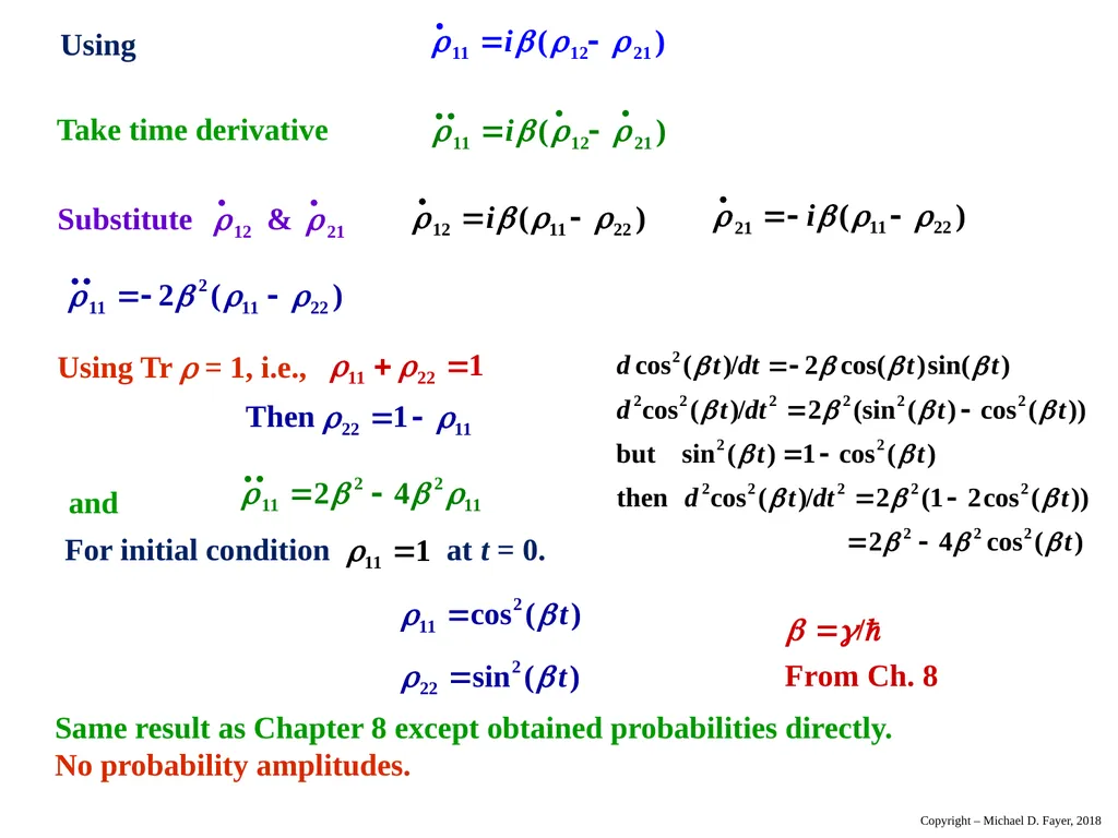
slide14. Using Take time derivative Same result as Chapter 8 except obtained probabilities directly.
No probability amplitudes. Copyright – Michael D. Fayer, 2018<br>
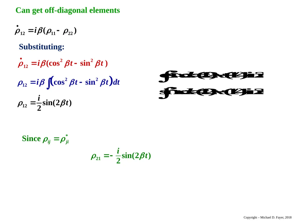
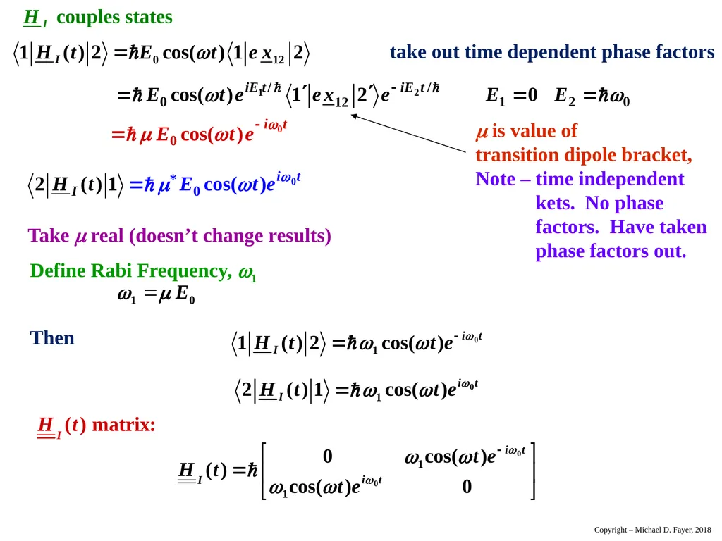
slide15. Can get off-diagonal elements Copyright – Michael D. Fayer, 2018<br>
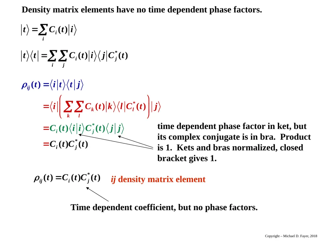
slide16. ij density matrix element Density matrix elements have no time dependent phase factors. time dependent phase factor in ket, but
its complex conjugate is in bra. Product
is 1. Kets and bras normalized, closed
bracket gives 1. Time dependent coefficient, but no phase factors. Copyright – Michael D. Fayer, 2018<br>
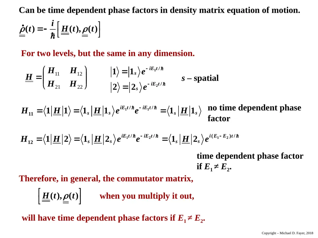
slide17. Can be time dependent phase factors in density matrix equation of motion. s – spatial no time dependent phase
factor time dependent phase factor
if E1 ≠ E2. Therefore, in general, the commutator matrix, will have time dependent phase factors if E1 ≠ E2. For two levels, but the same in any dimension. when you multiply it out, Copyright – Michael D. Fayer, 2018<br>
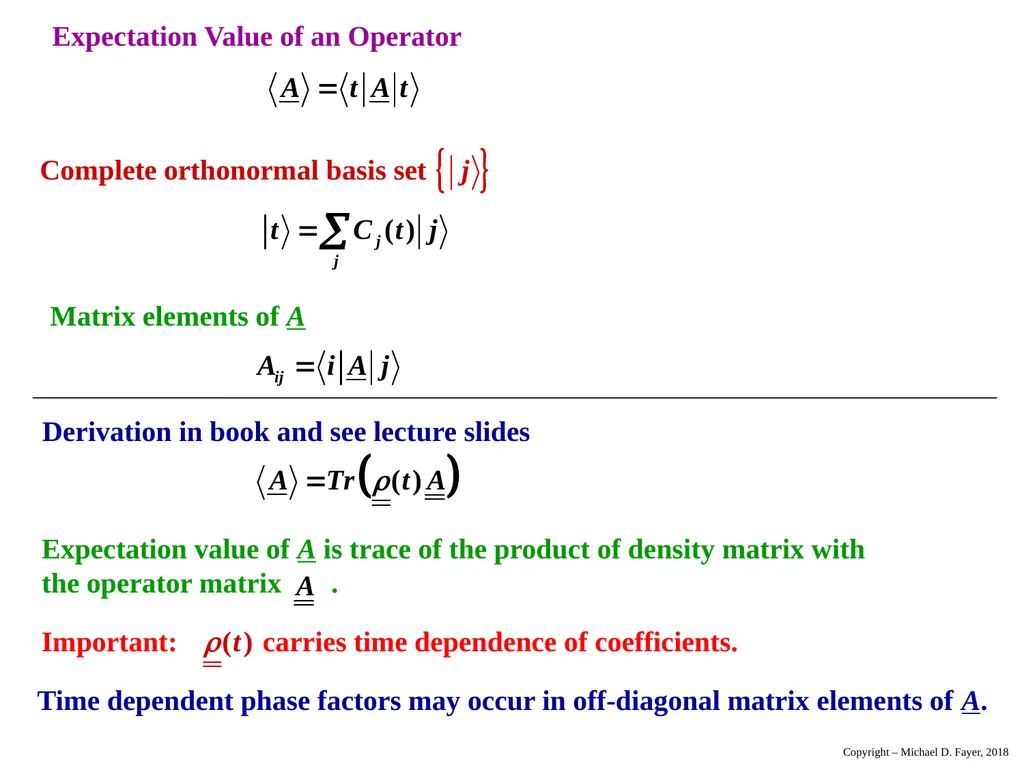
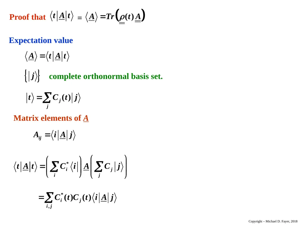
slide18. Expectation Value of an Operator Matrix elements of A Copyright – Michael D. Fayer, 2018<br>
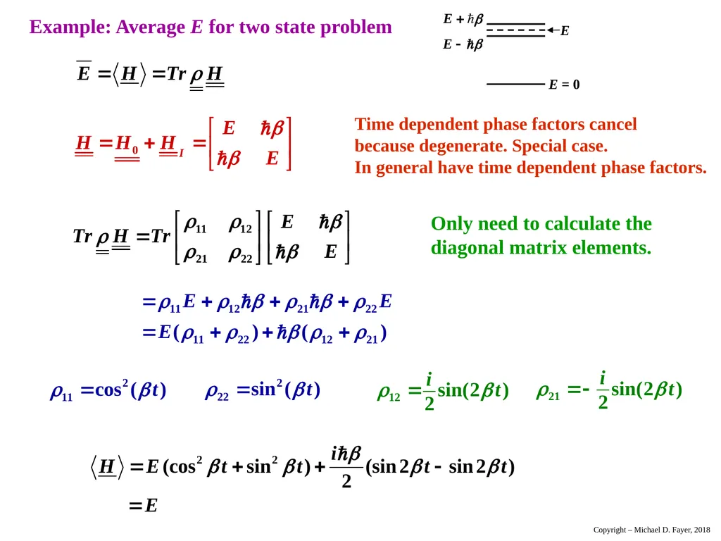
slide19. Example: Average E for two state problem Time dependent phase factors cancel
because degenerate. Special case.
In general have time dependent phase factors. E E = 0 Copyright – Michael D. Fayer, 2018<br>
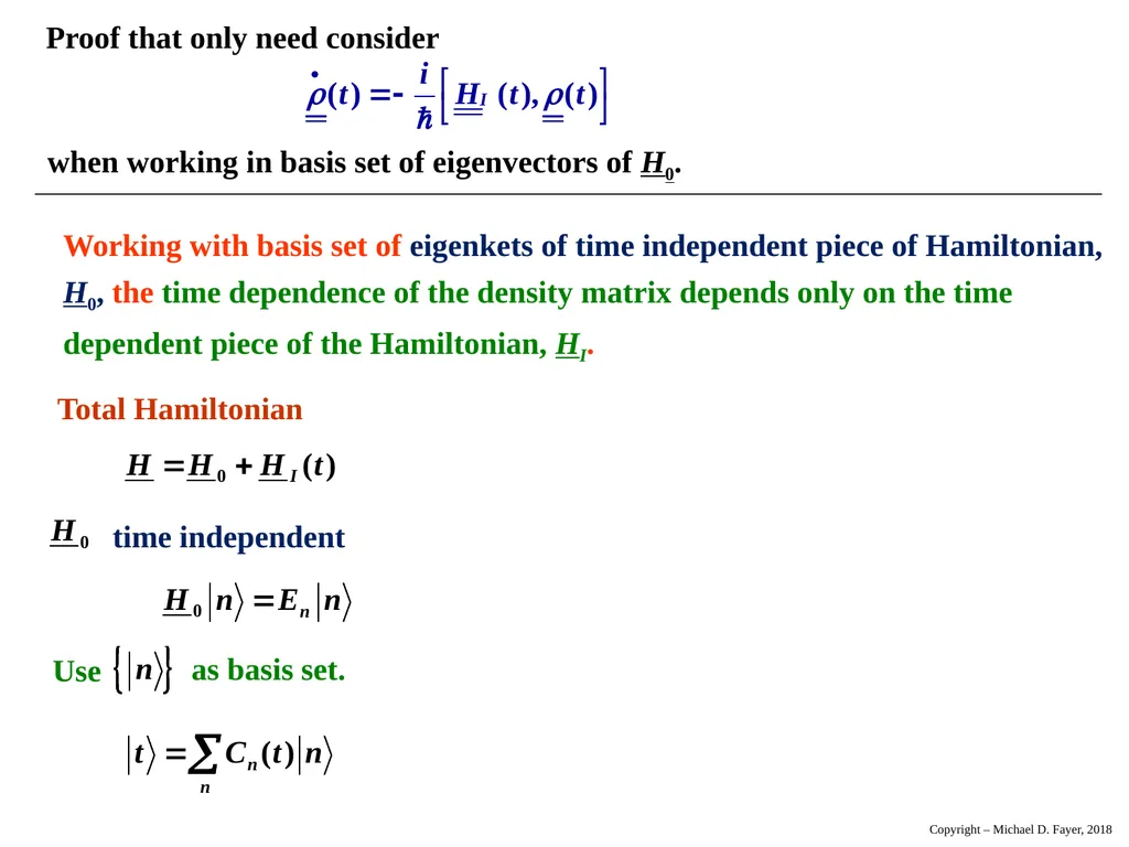
slide20. Working with basis set of eigenkets of time independent piece of Hamiltonian,
H0, the time dependence of the density matrix depends only on the time dependent piece of the Hamiltonian, HI. Copyright – Michael D. Fayer, 2018<br>
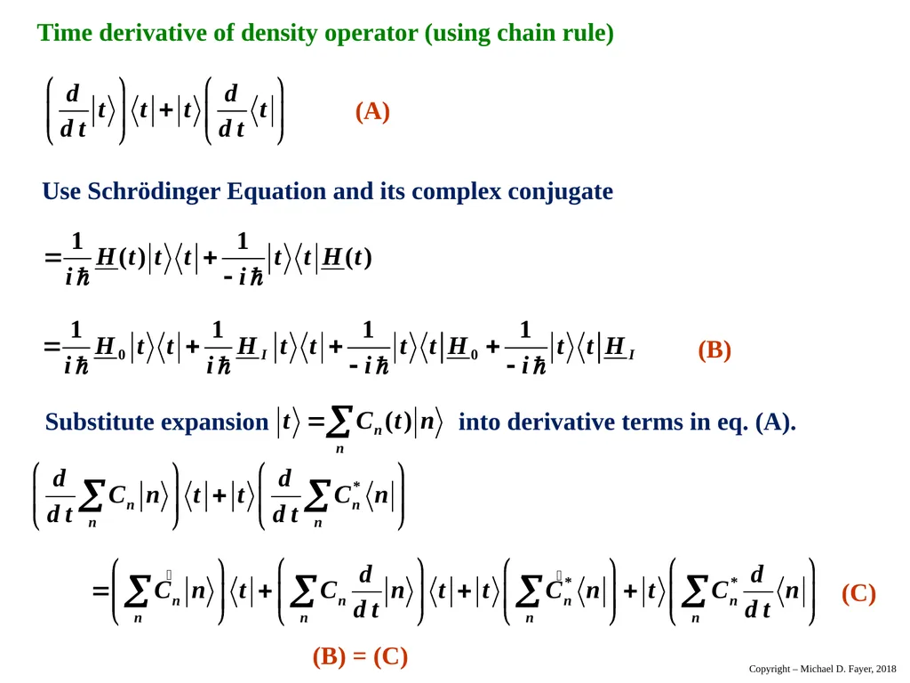
slide21. Time derivative of density operator (using chain rule) (A) Copyright – Michael D. Fayer, 2018<br>
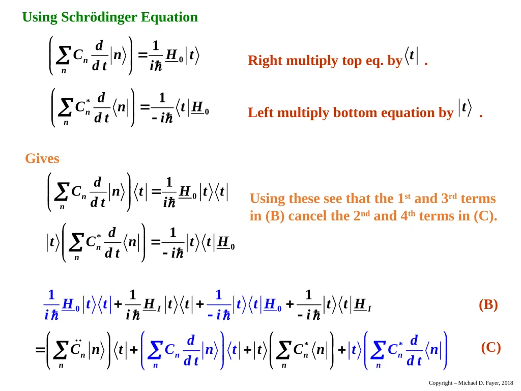
slide22. Using Schrödinger Equation Copyright – Michael D. Fayer, 2018<br>
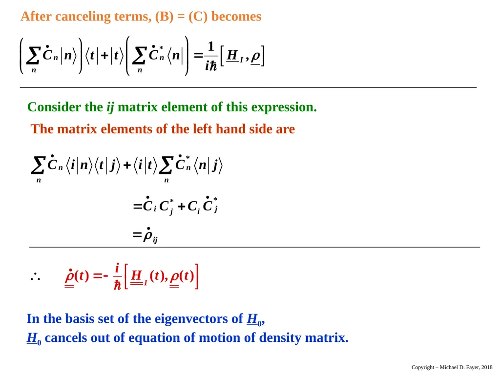
slide23. After canceling terms, (B) = (C) becomes Copyright – Michael D. Fayer, 2018<br>
slide24. Expectation value complete orthonormal basis set. Copyright – Michael D. Fayer, 2018<br>
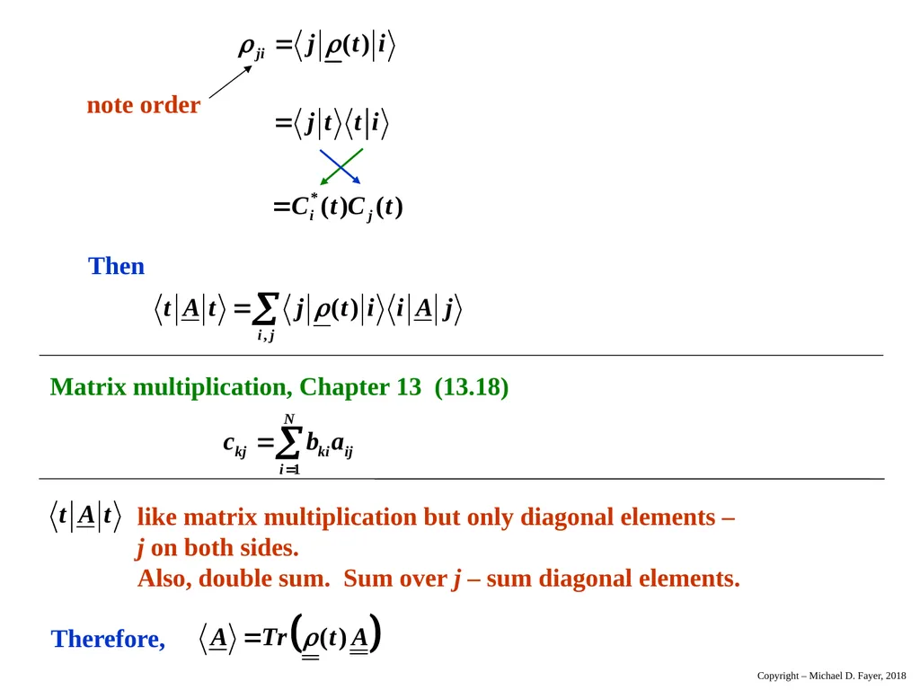
slide25. note order Then Copyright – Michael D. Fayer, 2018<br>
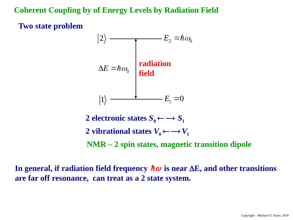
slide26. radiation
field Coherent Coupling by of Energy Levels by Radiation Field Two state problem In general, if radiation field frequency is near E, and other transitions
are far off resonance, can treat as a 2 state system. NMR – 2 spin states, magnetic transition dipole Copyright – Michael D. Fayer, 2018<br>
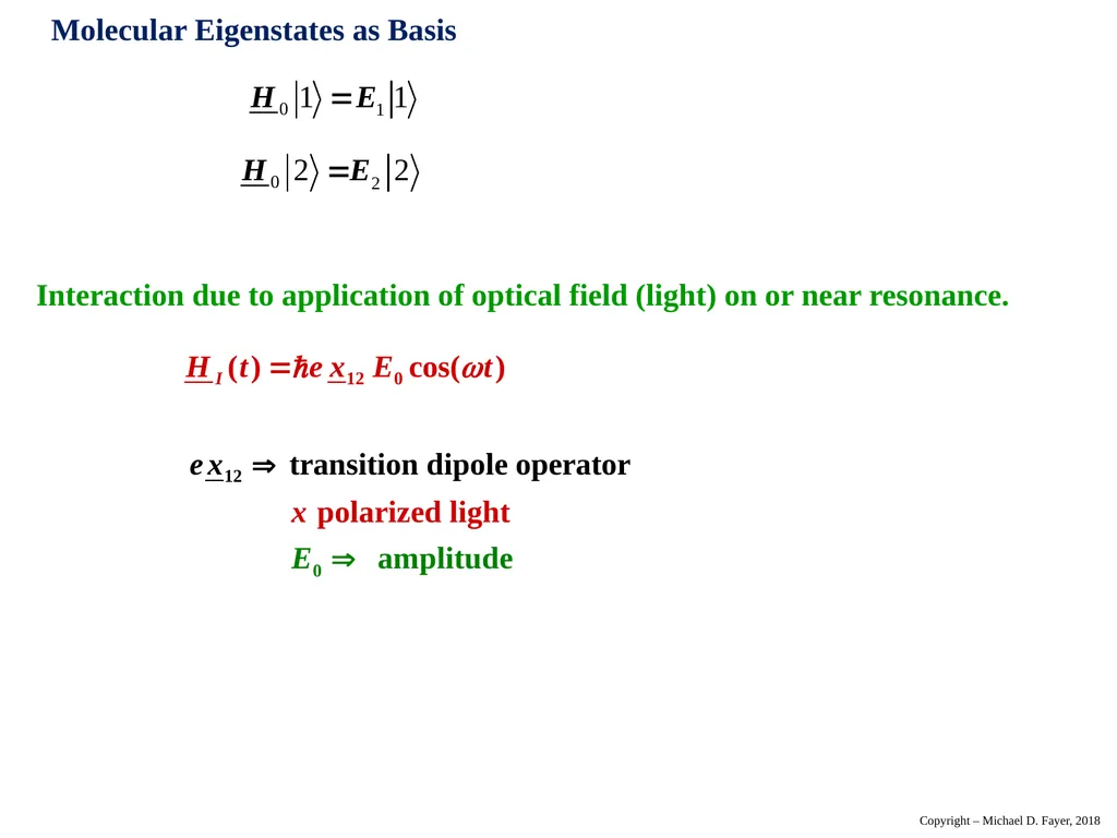
slide27. Molecular Eigenstates as Basis Interaction due to application of optical field (light) on or near resonance. Copyright – Michael D. Fayer, 2018<br>
slide28. Copyright – Michael D. Fayer, 2018<br>
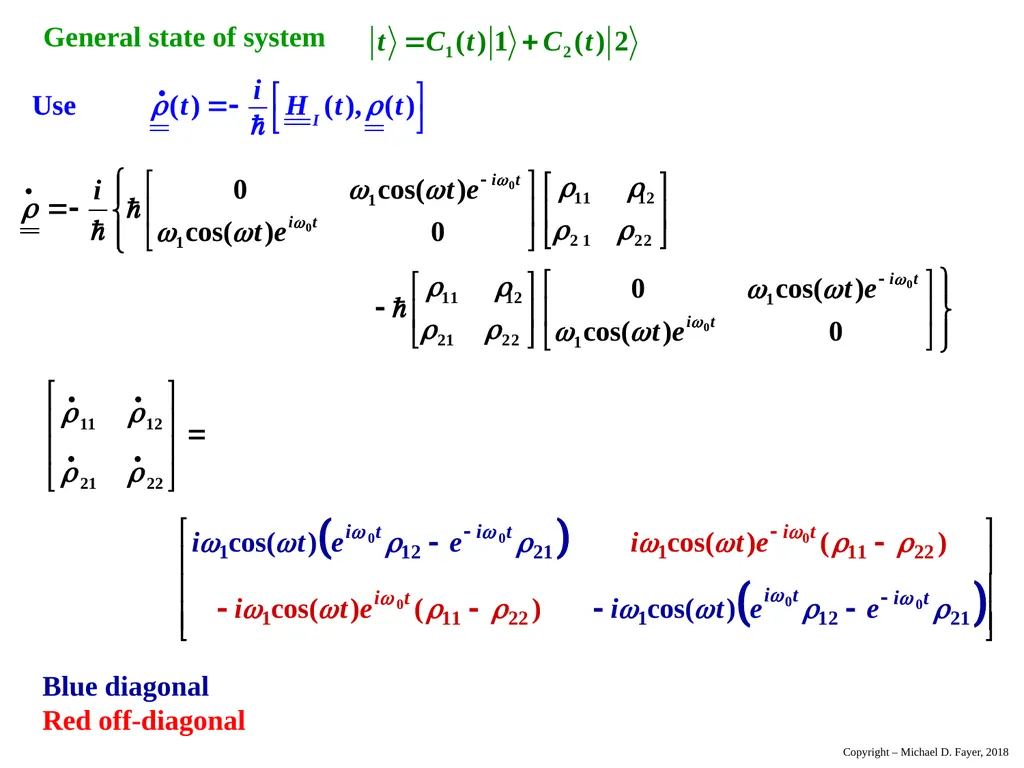
slide29. General state of system Copyright – Michael D. Fayer, 2018<br>
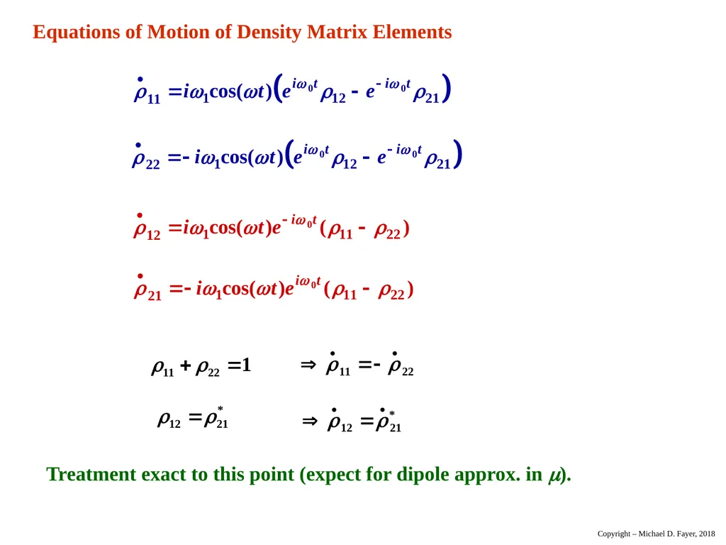
slide30. Equations of Motion of Density Matrix Elements Treatment exact to this point (expect for dipole approx. in ). Copyright – Michael D. Fayer, 2018<br>
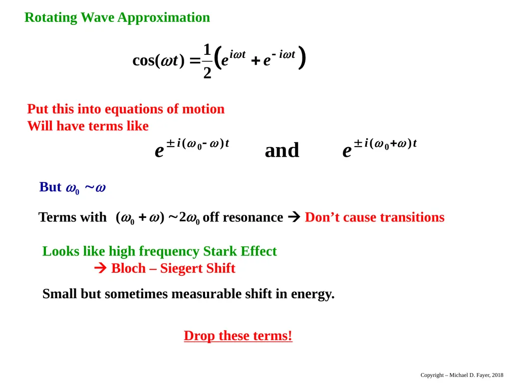
slide31. Rotating Wave Approximation Put this into equations of motion
Will have terms like Terms with off resonance Don’t cause transitions Looks like high frequency Stark Effect
Bloch – Siegert Shift Small but sometimes measurable shift in energy. Drop these terms! Copyright – Michael D. Fayer, 2018<br>
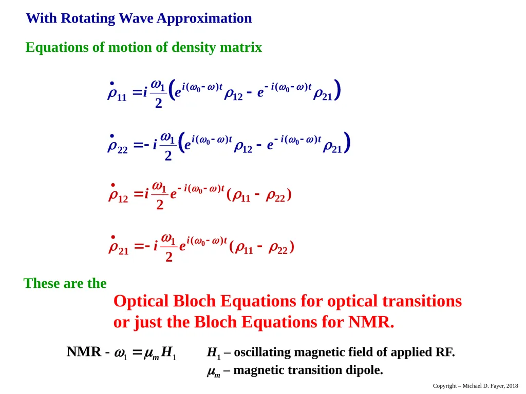
slide32. With Rotating Wave Approximation Equations of motion of density matrix These are the Optical Bloch Equations for optical transitions or just the Bloch Equations for NMR. Copyright – Michael D. Fayer, 2018 H1 – oscillating magnetic field of applied RF.
m – magnetic transition dipole.<br>
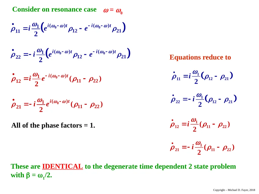
slide33. Consider on resonance case = 0 These are IDENTICAL to the degenerate time dependent 2 state problem with = 1/2. All of the phase factors = 1. Copyright – Michael D. Fayer, 2018<br>
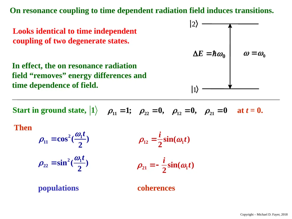
slide34. On resonance coupling to time dependent radiation field induces transitions. Looks identical to time independent
coupling of two degenerate states. In effect, the on resonance radiation
field “removes” energy differences and
time dependence of field. Then populations coherences at t = 0. Copyright – Michael D. Fayer, 2018<br>
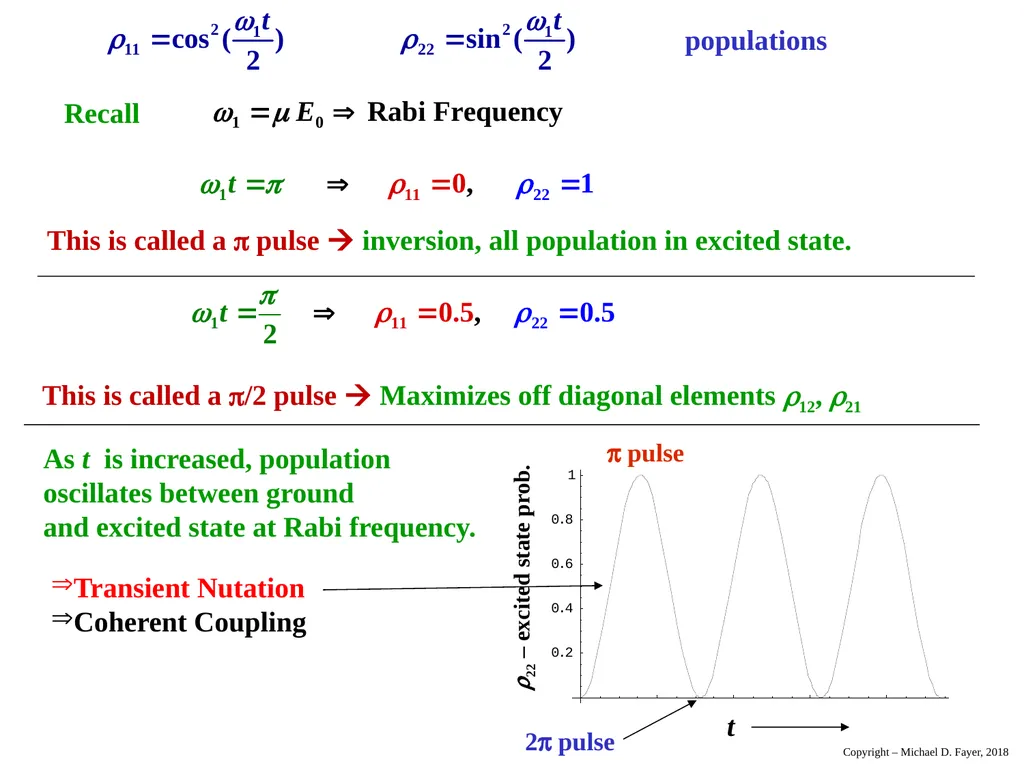
slide35. Recall This is called a pulse inversion, all population in excited state. populations Copyright – Michael D. Fayer, 2018<br>
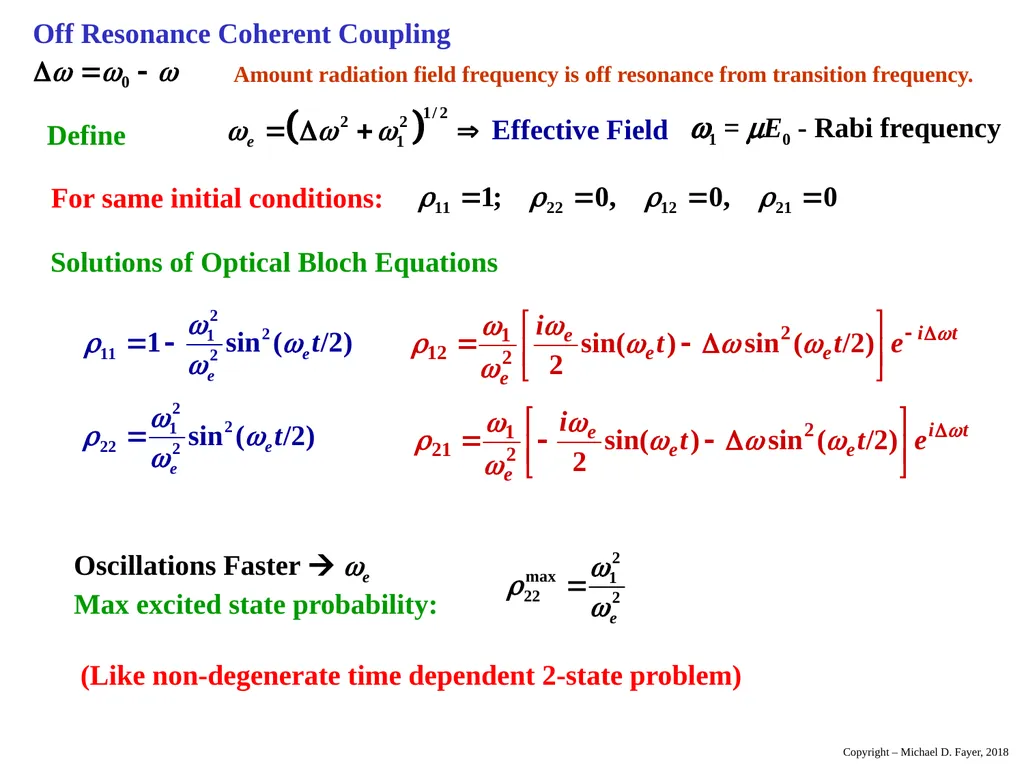
slide36. Off Resonance Coherent Coupling Define w1 = mE0 - Rabi frequency Amount radiation field frequency is off resonance from transition frequency. Copyright – Michael D. Fayer, 2018<br>
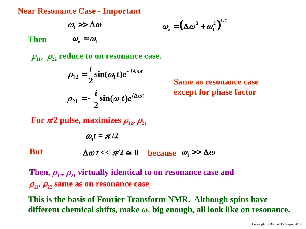
slide37. Near Resonance Case - Important Then 11, 22 reduce to on resonance case. This is the basis of Fourier Transform NMR. Although spins have
different chemical shifts, make ω1 big enough, all look like on resonance. Copyright – Michael D. Fayer, 2018<br>
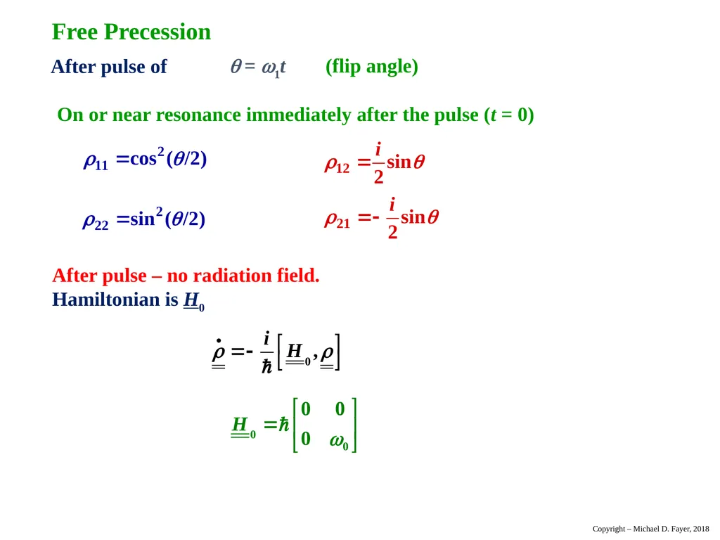
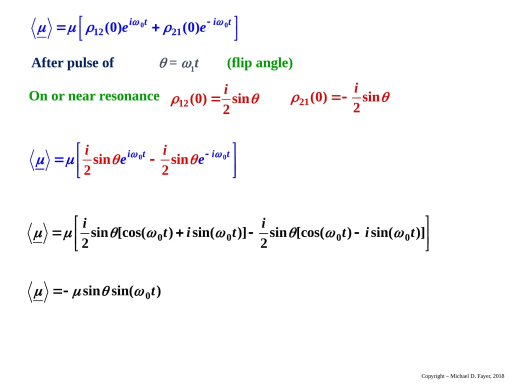
slide38. Free Precession After pulse of = 1t (flip angle) On or near resonance immediately after the pulse (t = 0) After pulse – no radiation field.
Hamiltonian is H0 Copyright – Michael D. Fayer, 2018<br>
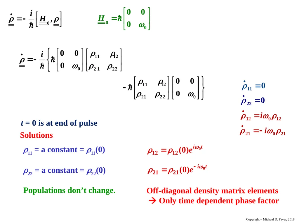
slide39. Copyright – Michael D. Fayer, 2018<br>
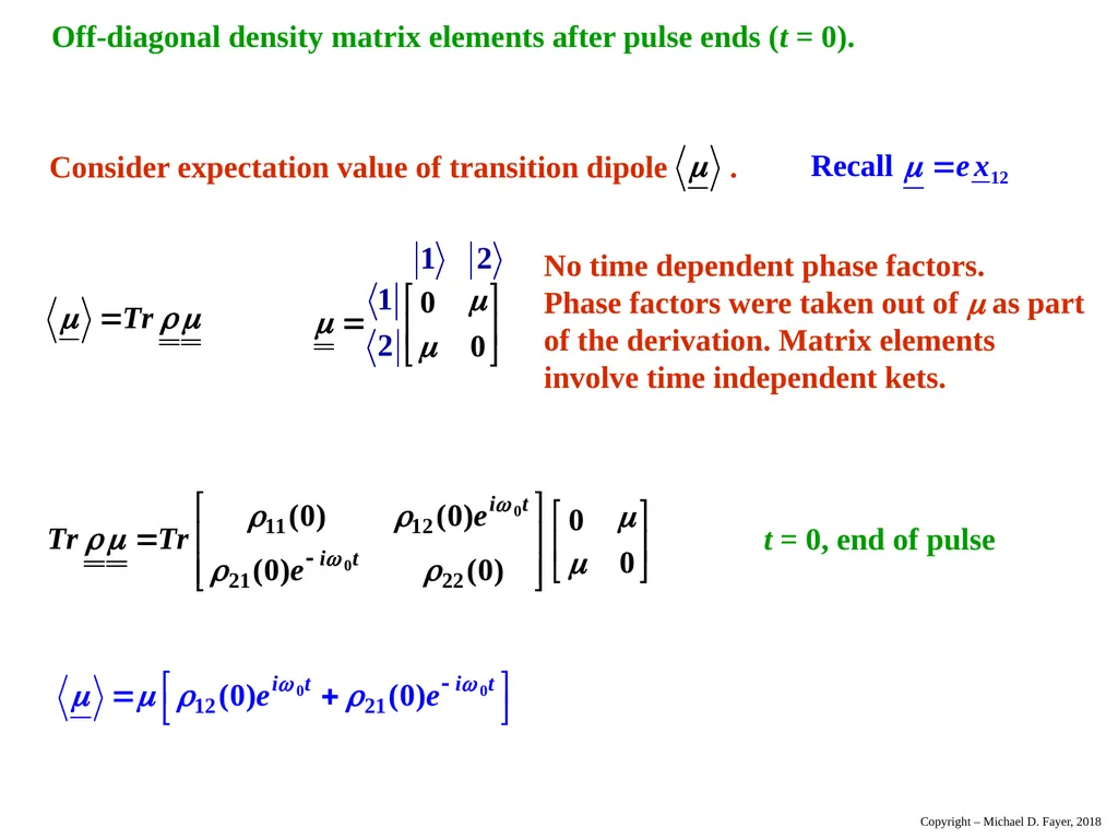
slide40. Off-diagonal density matrix elements after pulse ends (t = 0). Consider expectation value of transition dipole . No time dependent phase factors. Phase factors were taken out of as part of the derivation. Matrix elements involve time independent kets. Copyright – Michael D. Fayer, 2018<br>
slide41. After pulse of = 1t (flip angle) On or near resonance Copyright – Michael D. Fayer, 2018<br>
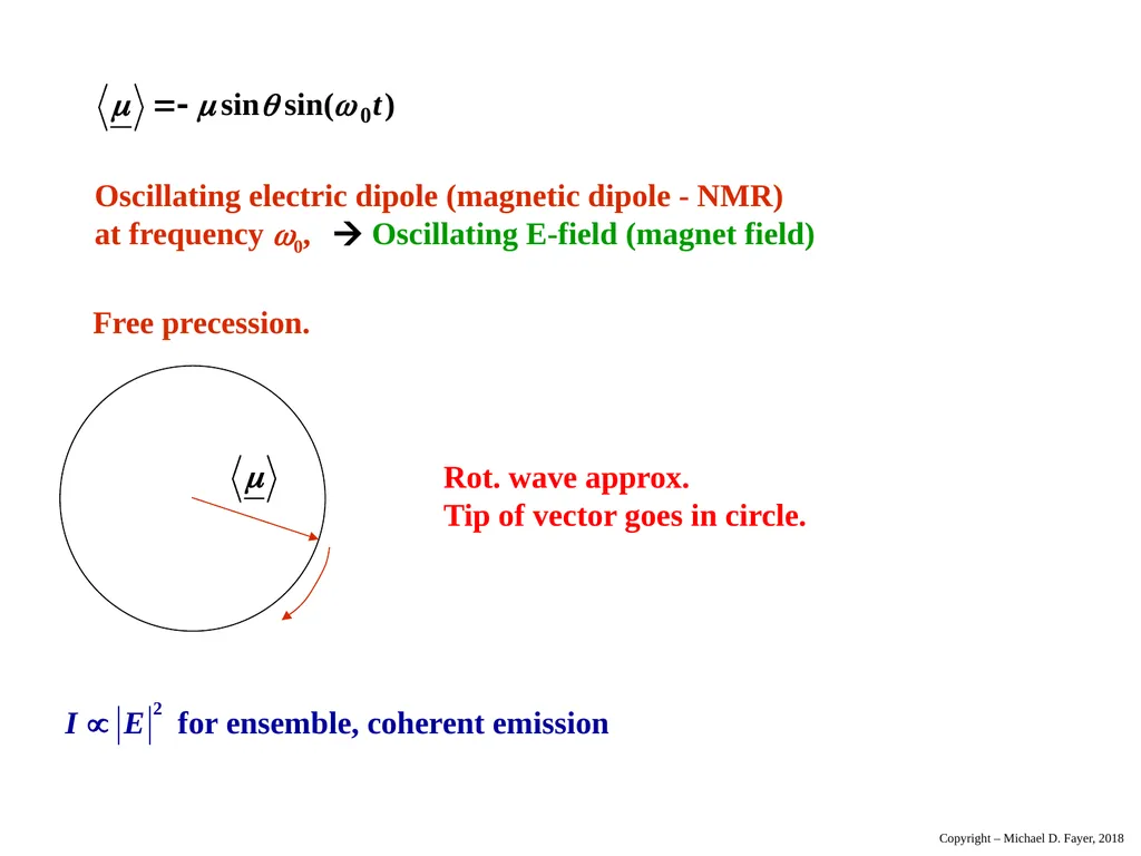
slide42. Oscillating electric dipole (magnetic dipole - NMR) at frequency 0, Oscillating E-field (magnet field) Free precession. Rot. wave approx.
Tip of vector goes in circle. Copyright – Michael D. Fayer, 2018<br>
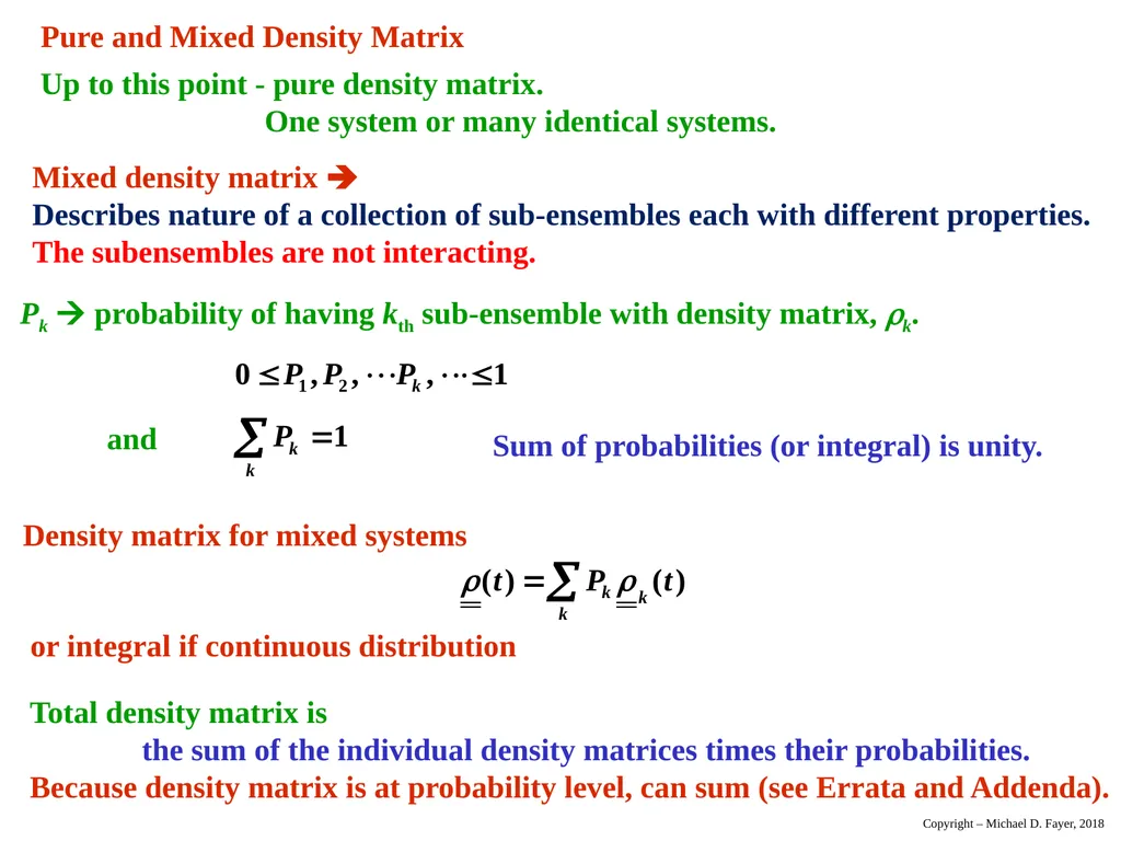
slide43. Pure and Mixed Density Matrix Up to this point - pure density matrix. One system or many identical systems. Mixed density matrix
Describes nature of a collection of sub-ensembles each with different properties.
The subensembles are not interacting. Copyright – Michael D. Fayer, 2018<br>
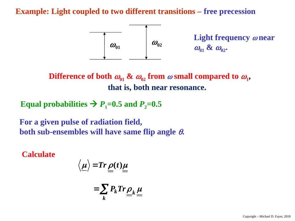
slide44. Example: Light coupled to two different transitions – free precession Difference of both 01 & 02 from small compared to 1, that is, both near resonance. Equal probabilities P1=0.5 and P2=0.5 Light frequency near 01 & 02. Copyright – Michael D. Fayer, 2018<br>
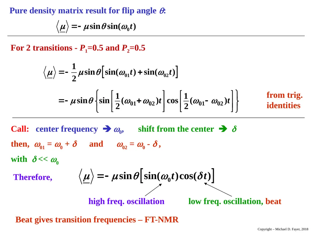
slide45. Pure density matrix result for flip angle : Copyright – Michael D. Fayer, 2018<br>
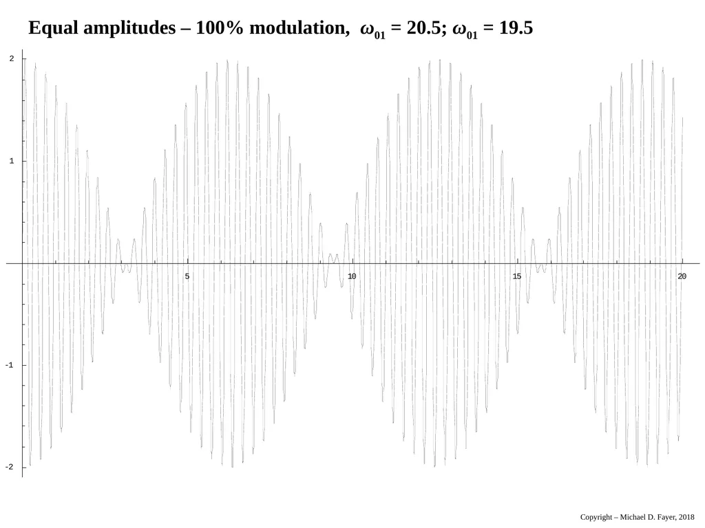
slide46. Equal amplitudes – 100% modulation, ω01 = 20.5; ω01 = 19.5 Copyright – Michael D. Fayer, 2018<br>
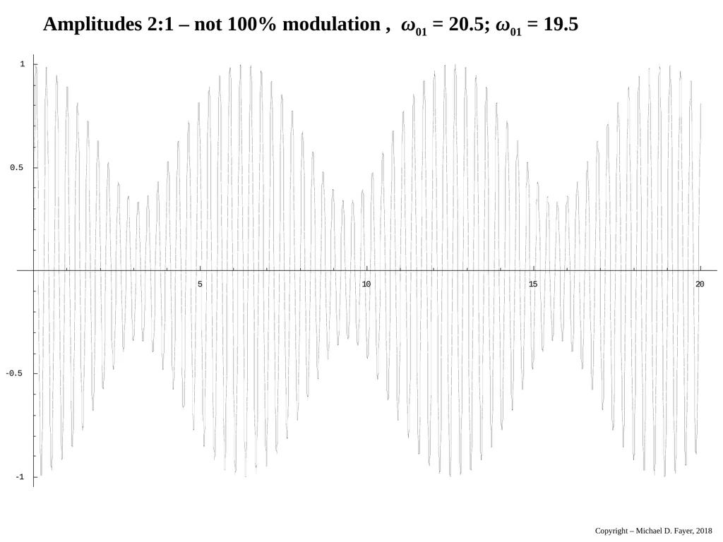
slide47. Amplitudes 2:1 – not 100% modulation , ω01 = 20.5; ω01 = 19.5 Copyright – Michael D. Fayer, 2018<br>
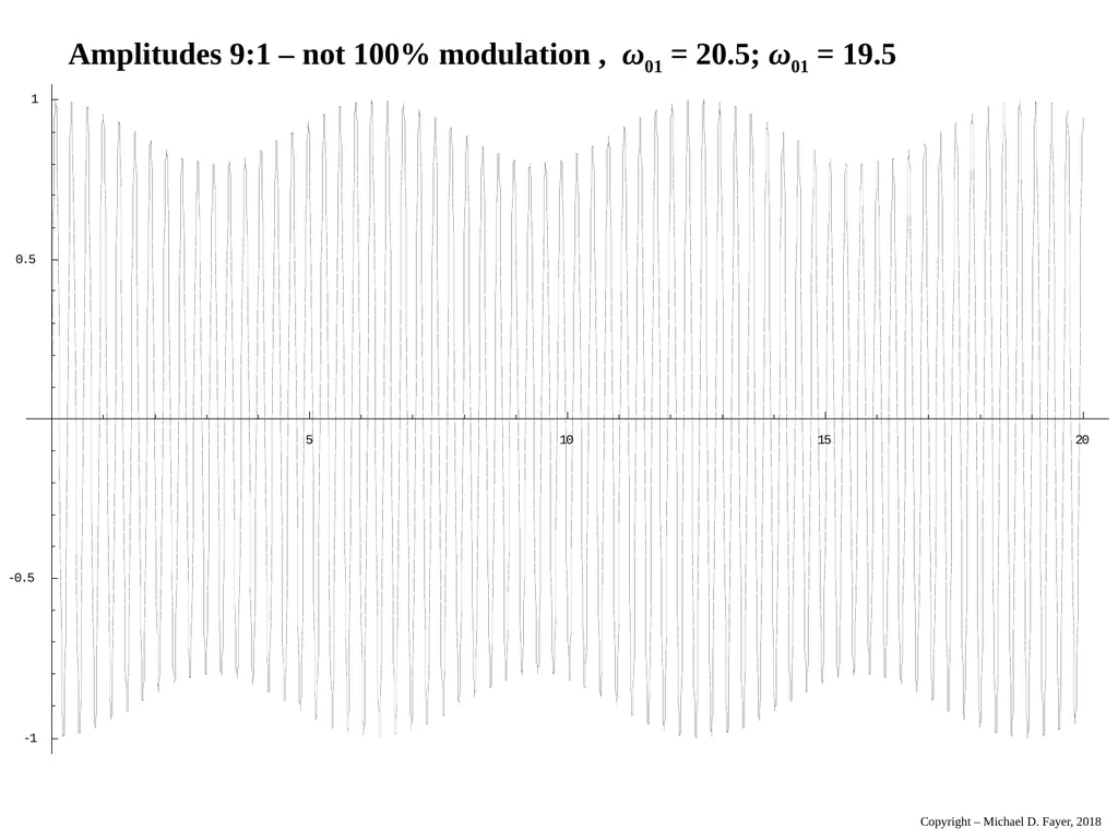
slide48. Amplitudes 9:1 – not 100% modulation , ω01 = 20.5; ω01 = 19.5 Copyright – Michael D. Fayer, 2018<br>
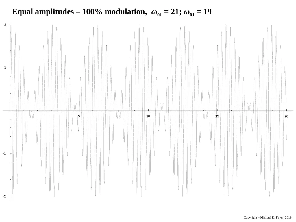
slide49. Equal amplitudes – 100% modulation, ω01 = 21; ω01 = 19 Copyright – Michael D. Fayer, 2018<br>
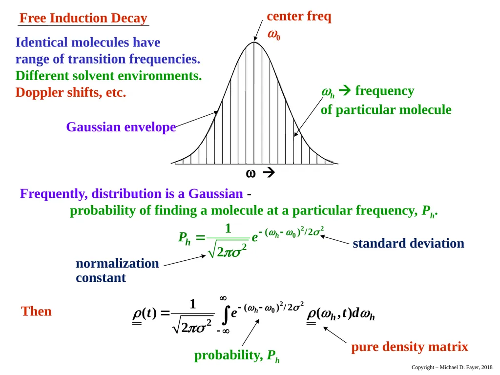
slide50. Free Induction Decay center freq
0 h frequency
of particular molecule w Frequently, distribution is a Gaussian - probability of finding a molecule at a particular frequency, Ph. Identical molecules have range of transition frequencies. Different solvent environments. Doppler shifts, etc. Gaussian envelope Copyright – Michael D. Fayer, 2018<br>
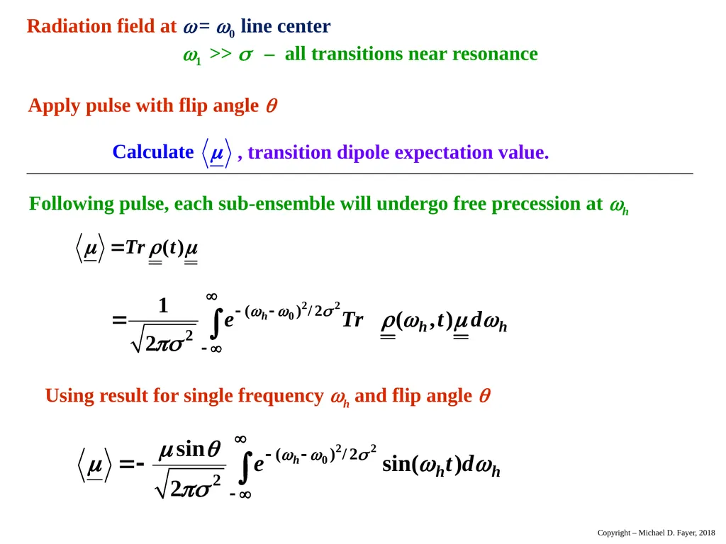
slide51. Radiation field at = 0 line center
1 >> – all transitions near resonance Apply pulse with flip angle , transition dipole expectation value. Copyright – Michael D. Fayer, 2018<br>
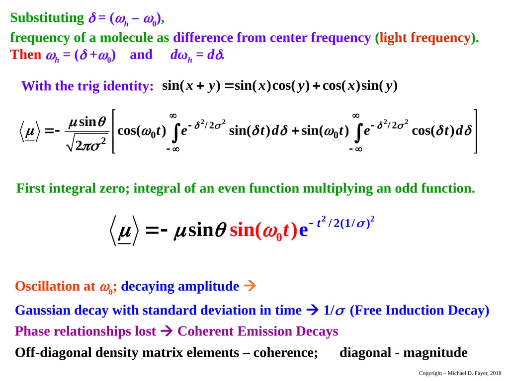
slide52. Substituting = (h – 0), frequency of a molecule as difference from center frequency (light frequency).
Then h = ( +0) and dωh = d. Copyright – Michael D. Fayer, 2018<br>
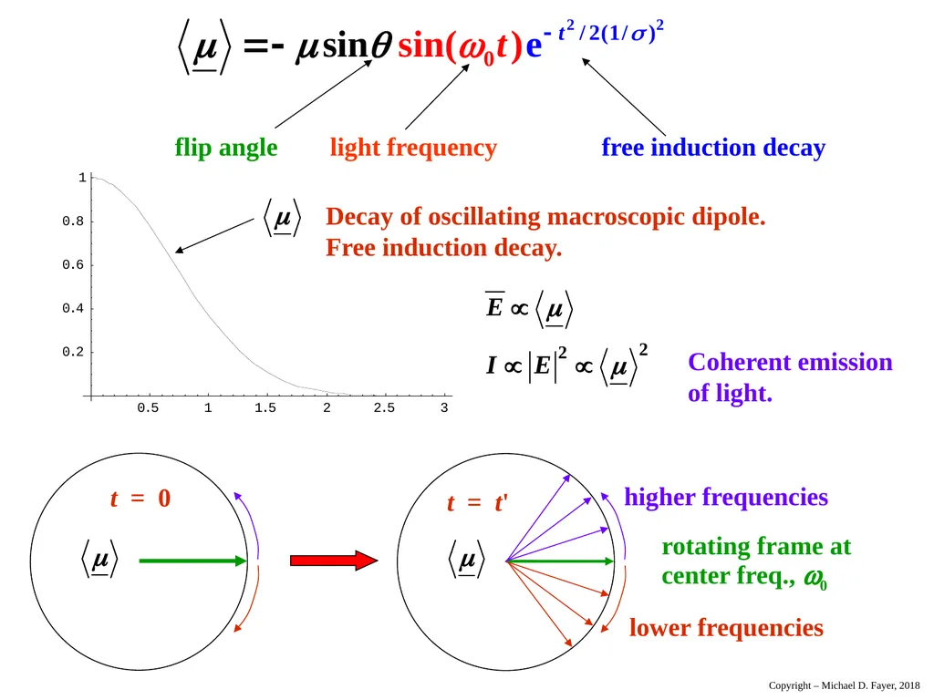
slide53. flip angle light frequency free induction decay Copyright – Michael D. Fayer, 2018<br>
slide2. Density Matrix State of a system at time t: Contains time dependent
phase factors. Copyright – Michael D. Fayer, 2018<br>
slide3. Two state system: Copyright – Michael D. Fayer, 2018<br>
slide4. In general: ij density matrix element Copyright – Michael D. Fayer, 2018<br>
slide5. 2×2 Density Matrix: Diagonal density matrix elements probs. of finding system in various states
Off Diagonal Elements “coherences” Copyright – Michael D. Fayer, 2018<br>
slide6. Time dependence of product rule Copyright – Michael D. Fayer, 2018<br>
slide7. Substituting: density operator Copyright – Michael D. Fayer, 2018<br>
slide8. Density Matrix Equations of Motion by product rule time derivative of density matrix elements Copyright – Michael D. Fayer, 2018<br>
slide9. Copyright – Michael D. Fayer, 2018<br>
slide10. In many problems: time
independent time
dependent e.g., Molecule in a radiation field: Copyright – Michael D. Fayer, 2018<br>
slide11. For this situation: time evolution of density matrix elements, Cij(t), depends only on time dependent interaction term See derivation in book – and lecture slides.
Like first steps in time dependent perturbation theory before any approximations. In absence of , only time dependence from time dependent phase factors
from . No changes in magnitudes of coefficients Cij . Copyright – Michael D. Fayer, 2018<br>
slide12. Time Dependent Two State Problem Revisited: Previously treated in Chapter 8 with Schrödinger Equation. Copyright – Michael D. Fayer, 2018<br>
slide13. Use Copyright – Michael D. Fayer, 2018<br>
slide14. Using Take time derivative Same result as Chapter 8 except obtained probabilities directly.
No probability amplitudes. Copyright – Michael D. Fayer, 2018<br>
slide15. Can get off-diagonal elements Copyright – Michael D. Fayer, 2018<br>
slide16. ij density matrix element Density matrix elements have no time dependent phase factors. time dependent phase factor in ket, but
its complex conjugate is in bra. Product
is 1. Kets and bras normalized, closed
bracket gives 1. Time dependent coefficient, but no phase factors. Copyright – Michael D. Fayer, 2018<br>
slide17. Can be time dependent phase factors in density matrix equation of motion. s – spatial no time dependent phase
factor time dependent phase factor
if E1 ≠ E2. Therefore, in general, the commutator matrix, will have time dependent phase factors if E1 ≠ E2. For two levels, but the same in any dimension. when you multiply it out, Copyright – Michael D. Fayer, 2018<br>
slide18. Expectation Value of an Operator Matrix elements of A Copyright – Michael D. Fayer, 2018<br>
slide19. Example: Average E for two state problem Time dependent phase factors cancel
because degenerate. Special case.
In general have time dependent phase factors. E E = 0 Copyright – Michael D. Fayer, 2018<br>
slide20. Working with basis set of eigenkets of time independent piece of Hamiltonian,
H0, the time dependence of the density matrix depends only on the time dependent piece of the Hamiltonian, HI. Copyright – Michael D. Fayer, 2018<br>
slide21. Time derivative of density operator (using chain rule) (A) Copyright – Michael D. Fayer, 2018<br>
slide22. Using Schrödinger Equation Copyright – Michael D. Fayer, 2018<br>
slide23. After canceling terms, (B) = (C) becomes Copyright – Michael D. Fayer, 2018<br>
slide24. Expectation value complete orthonormal basis set. Copyright – Michael D. Fayer, 2018<br>
slide25. note order Then Copyright – Michael D. Fayer, 2018<br>
slide26. radiation
field Coherent Coupling by of Energy Levels by Radiation Field Two state problem In general, if radiation field frequency is near E, and other transitions
are far off resonance, can treat as a 2 state system. NMR – 2 spin states, magnetic transition dipole Copyright – Michael D. Fayer, 2018<br>
slide27. Molecular Eigenstates as Basis Interaction due to application of optical field (light) on or near resonance. Copyright – Michael D. Fayer, 2018<br>
slide28. Copyright – Michael D. Fayer, 2018<br>
slide29. General state of system Copyright – Michael D. Fayer, 2018<br>
slide30. Equations of Motion of Density Matrix Elements Treatment exact to this point (expect for dipole approx. in ). Copyright – Michael D. Fayer, 2018<br>
slide31. Rotating Wave Approximation Put this into equations of motion
Will have terms like Terms with off resonance Don’t cause transitions Looks like high frequency Stark Effect
Bloch – Siegert Shift Small but sometimes measurable shift in energy. Drop these terms! Copyright – Michael D. Fayer, 2018<br>
slide32. With Rotating Wave Approximation Equations of motion of density matrix These are the Optical Bloch Equations for optical transitions or just the Bloch Equations for NMR. Copyright – Michael D. Fayer, 2018 H1 – oscillating magnetic field of applied RF.
m – magnetic transition dipole.<br>
slide33. Consider on resonance case = 0 These are IDENTICAL to the degenerate time dependent 2 state problem with = 1/2. All of the phase factors = 1. Copyright – Michael D. Fayer, 2018<br>
slide34. On resonance coupling to time dependent radiation field induces transitions. Looks identical to time independent
coupling of two degenerate states. In effect, the on resonance radiation
field “removes” energy differences and
time dependence of field. Then populations coherences at t = 0. Copyright – Michael D. Fayer, 2018<br>
slide35. Recall This is called a pulse inversion, all population in excited state. populations Copyright – Michael D. Fayer, 2018<br>
slide36. Off Resonance Coherent Coupling Define w1 = mE0 - Rabi frequency Amount radiation field frequency is off resonance from transition frequency. Copyright – Michael D. Fayer, 2018<br>
slide37. Near Resonance Case - Important Then 11, 22 reduce to on resonance case. This is the basis of Fourier Transform NMR. Although spins have
different chemical shifts, make ω1 big enough, all look like on resonance. Copyright – Michael D. Fayer, 2018<br>
slide38. Free Precession After pulse of = 1t (flip angle) On or near resonance immediately after the pulse (t = 0) After pulse – no radiation field.
Hamiltonian is H0 Copyright – Michael D. Fayer, 2018<br>
slide39. Copyright – Michael D. Fayer, 2018<br>
slide40. Off-diagonal density matrix elements after pulse ends (t = 0). Consider expectation value of transition dipole . No time dependent phase factors. Phase factors were taken out of as part of the derivation. Matrix elements involve time independent kets. Copyright – Michael D. Fayer, 2018<br>
slide41. After pulse of = 1t (flip angle) On or near resonance Copyright – Michael D. Fayer, 2018<br>
slide42. Oscillating electric dipole (magnetic dipole - NMR) at frequency 0, Oscillating E-field (magnet field) Free precession. Rot. wave approx.
Tip of vector goes in circle. Copyright – Michael D. Fayer, 2018<br>
slide43. Pure and Mixed Density Matrix Up to this point - pure density matrix. One system or many identical systems. Mixed density matrix
Describes nature of a collection of sub-ensembles each with different properties.
The subensembles are not interacting. Copyright – Michael D. Fayer, 2018<br>
slide44. Example: Light coupled to two different transitions – free precession Difference of both 01 & 02 from small compared to 1, that is, both near resonance. Equal probabilities P1=0.5 and P2=0.5 Light frequency near 01 & 02. Copyright – Michael D. Fayer, 2018<br>
slide45. Pure density matrix result for flip angle : Copyright – Michael D. Fayer, 2018<br>
slide46. Equal amplitudes – 100% modulation, ω01 = 20.5; ω01 = 19.5 Copyright – Michael D. Fayer, 2018<br>
slide47. Amplitudes 2:1 – not 100% modulation , ω01 = 20.5; ω01 = 19.5 Copyright – Michael D. Fayer, 2018<br>
slide48. Amplitudes 9:1 – not 100% modulation , ω01 = 20.5; ω01 = 19.5 Copyright – Michael D. Fayer, 2018<br>
slide49. Equal amplitudes – 100% modulation, ω01 = 21; ω01 = 19 Copyright – Michael D. Fayer, 2018<br>
slide50. Free Induction Decay center freq
0 h frequency
of particular molecule w Frequently, distribution is a Gaussian - probability of finding a molecule at a particular frequency, Ph. Identical molecules have range of transition frequencies. Different solvent environments. Doppler shifts, etc. Gaussian envelope Copyright – Michael D. Fayer, 2018<br>
slide51. Radiation field at = 0 line center
1 >> – all transitions near resonance Apply pulse with flip angle , transition dipole expectation value. Copyright – Michael D. Fayer, 2018<br>
slide52. Substituting = (h – 0), frequency of a molecule as difference from center frequency (light frequency).
Then h = ( +0) and dωh = d. Copyright – Michael D. Fayer, 2018<br>
slide53. flip angle light frequency free induction decay Copyright – Michael D. Fayer, 2018<br>