
Chapter 22: Parallel and Distributed Query

Description: Chapter 22: Parallel and Distributed Query Processing Chapter 22: Parallel And Distributed Query Processing Overview Parallel Sort Parallel Join Other Operations Parallel Evaluation of Query Plans Query Processing on Shared Memory Query
Related Topics
Download Presentation
"Chapter 22: Parallel and Distributed Query" is the property of its rightful owner. Permission is granted to download and print the materials on this website for personal, non-commercial use only, and to display it on your personal computer provided you do not modify the materials and that you retain all copyright notices contained in the materials. By downloading content from our website, you accept the terms of this agreement.
Presentation Transcript
slide1. Chapter 22: Parallel and Distributed Query Processing<br>
slide2. Chapter 22: Parallel And Distributed Query Processing Overview
Parallel Sort
Parallel Join
Other Operations
Parallel Evaluation of Query Plans
Query Processing on Shared Memory
Query Optimization
Distributed Query Processing<br>
slide3. Parallel Query Processing Different queries/transactions can be run in parallel with each other.
Interquery parallelism
Concurrency control takes care of conflicts in case of updates
More on parallel transaction processing in Chapter 23
Focus in this chapter is on read-only queries
Individual relational operations (e.g., sort, join, aggregation) can be executed in parallel
data can be partitioned and each processor can work independently on its own partition.
Queries are expressed in high level language (SQL, translated to relational algebra)
makes parallelization easier.<br>
slide4. Intraquery Parallelism Intraquery parallelism: execution of a single query in parallel on multiple processors/disks; important for speeding up long-running queries.
Two complementary forms of intraquery parallelism:
Intraoperation Parallelism – parallelize the execution of each individual operation in the query
Supports high degree of parallelism
Interoperation Parallelism – execute the different operations in a query expression in parallel.
Limited degree of parallelism<br>
slide5. Parallel Processing of Relational Operations Our discussion of parallel algorithms assumes:
read-only queries
shared-nothing architecture
n nodes, N1, ..., Nn
Each assumed to have disks and processors.
Initial focus on parallelization to a shared-nothing node
Parallel processing within a shared memory/shared disk node discussed later
Shared-nothing architectures can be efficiently simulated on shared-memory and shared-disk systems.
Algorithms for shared-nothing systems can thus be run on shared-memory and shared-disk systems.
However, some optimizations may be possible.<br>
slide6. Intraoperation Parallelism<br>
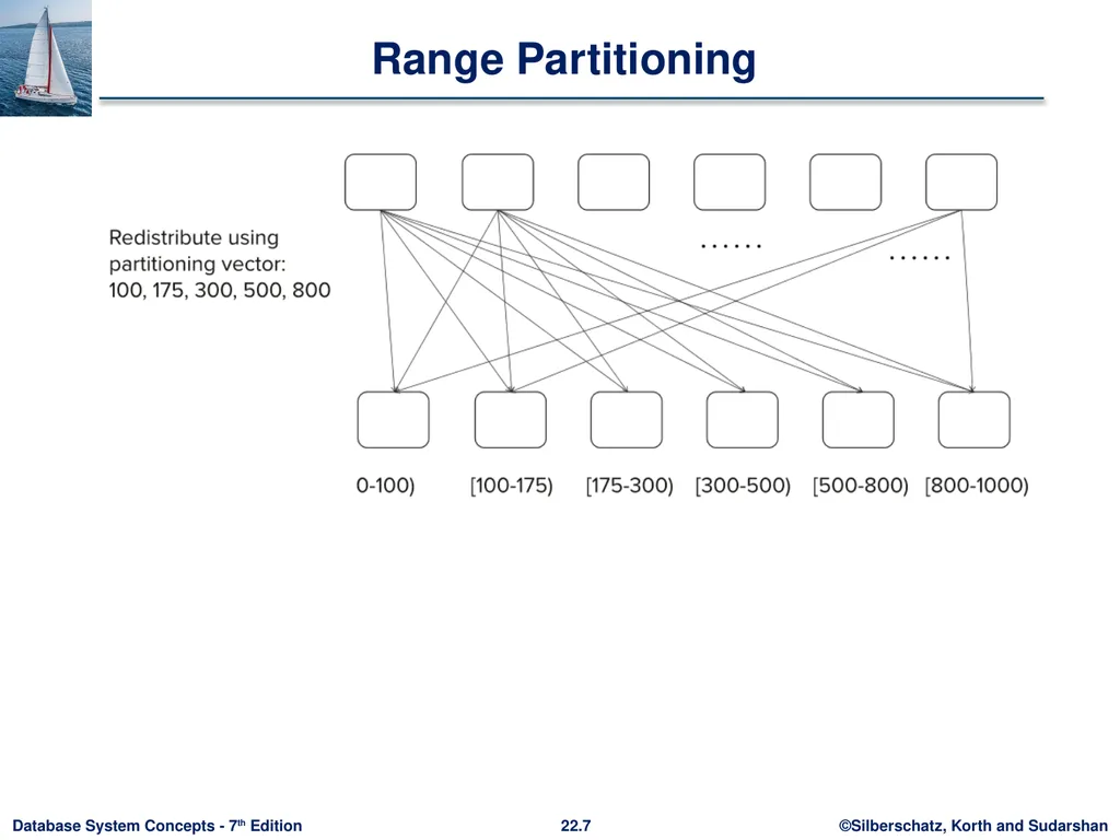
slide7. Range Partitioning<br>
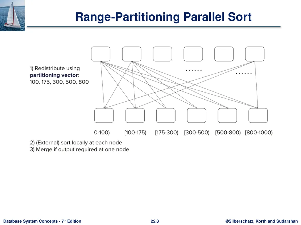
slide8. Range-Partitioning Parallel Sort<br>
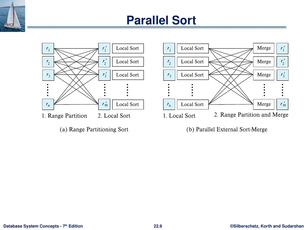
slide9. Parallel Sort<br>
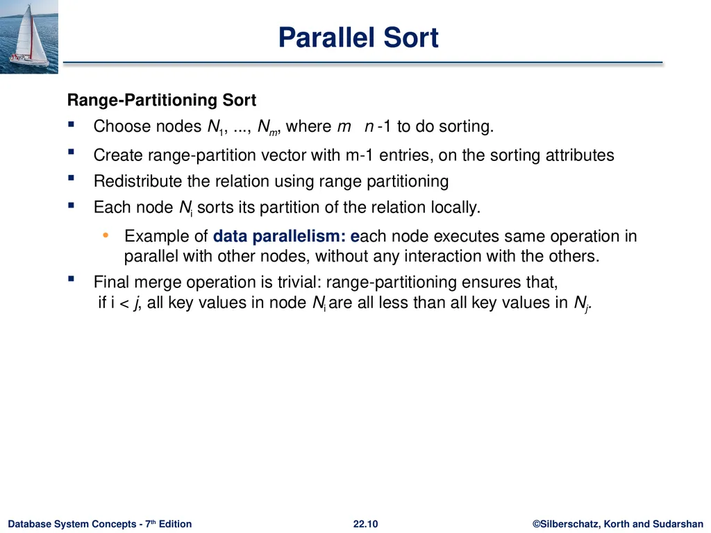
slide10. Parallel Sort Range-Partitioning Sort
Choose nodes N1, ..., Nm, where m n -1 to do sorting.
Create range-partition vector with m-1 entries, on the sorting attributes
Redistribute the relation using range partitioning
Each node Ni sorts its partition of the relation locally.
Example of data parallelism: each node executes same operation in parallel with other nodes, without any interaction with the others.
Final merge operation is trivial: range-partitioning ensures that, if i < j, all key values in node Ni are all less than all key values in Nj.<br>
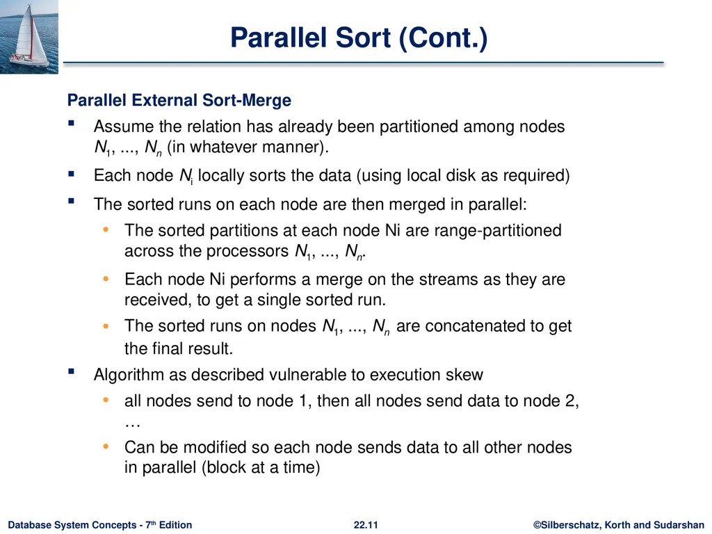
slide11. Parallel Sort (Cont.) Parallel External Sort-Merge
Assume the relation has already been partitioned among nodes N1, ..., Nn (in whatever manner).
Each node Ni locally sorts the data (using local disk as required)
The sorted runs on each node are then merged in parallel:
The sorted partitions at each node Ni are range-partitioned across the processors N1, ..., Nn.
Each node Ni performs a merge on the streams as they are received, to get a single sorted run.
The sorted runs on nodes N1, ..., Nn are concatenated to get the final result.
Algorithm as described vulnerable to execution skew
all nodes send to node 1, then all nodes send data to node 2, …
Can be modified so each node sends data to all other nodes in parallel (block at a time)<br>
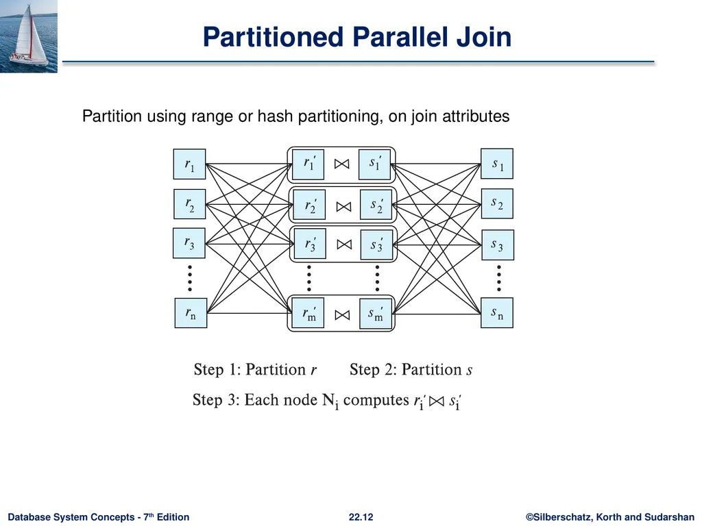
slide12. Partitioned Parallel Join Partition using range or hash partitioning, on join attributes<br>
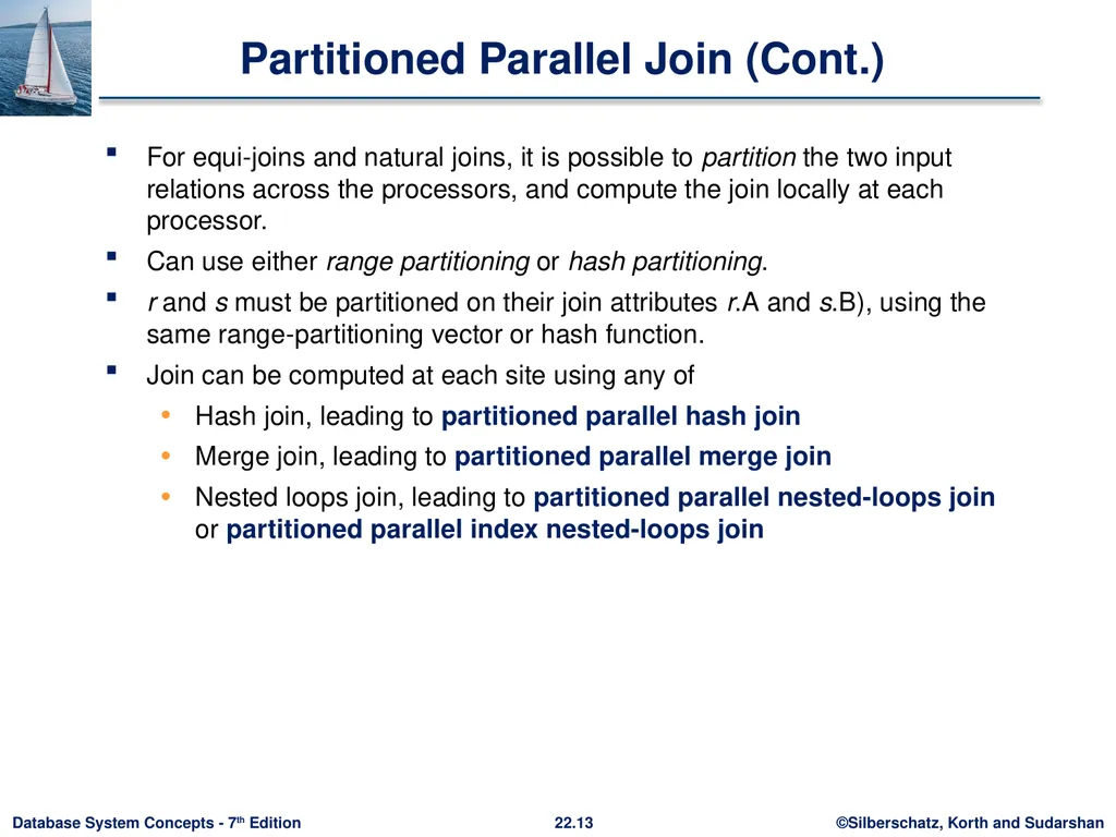
slide13. Partitioned Parallel Join (Cont.) For equi-joins and natural joins, it is possible to partition the two input relations across the processors, and compute the join locally at each processor.
Can use either range partitioning or hash partitioning.
r and s must be partitioned on their join attributes r.A and s.B), using the same range-partitioning vector or hash function.
Join can be computed at each site using any of
Hash join, leading to partitioned parallel hash join
Merge join, leading to partitioned parallel merge join
Nested loops join, leading to partitioned parallel nested-loops join or partitioned parallel index nested-loops join<br>
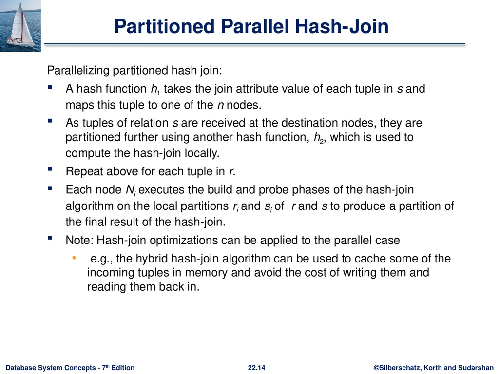
slide14. Partitioned Parallel Hash-Join Parallelizing partitioned hash join:
A hash function h1 takes the join attribute value of each tuple in s and maps this tuple to one of the n nodes.
As tuples of relation s are received at the destination nodes, they are partitioned further using another hash function, h2, which is used to compute the hash-join locally.
Repeat above for each tuple in r.
Each node Ni executes the build and probe phases of the hash-join algorithm on the local partitions ri and si of r and s to produce a partition of the final result of the hash-join.
Note: Hash-join optimizations can be applied to the parallel case
e.g., the hybrid hash-join algorithm can be used to cache some of the incoming tuples in memory and avoid the cost of writing them and reading them back in.<br>
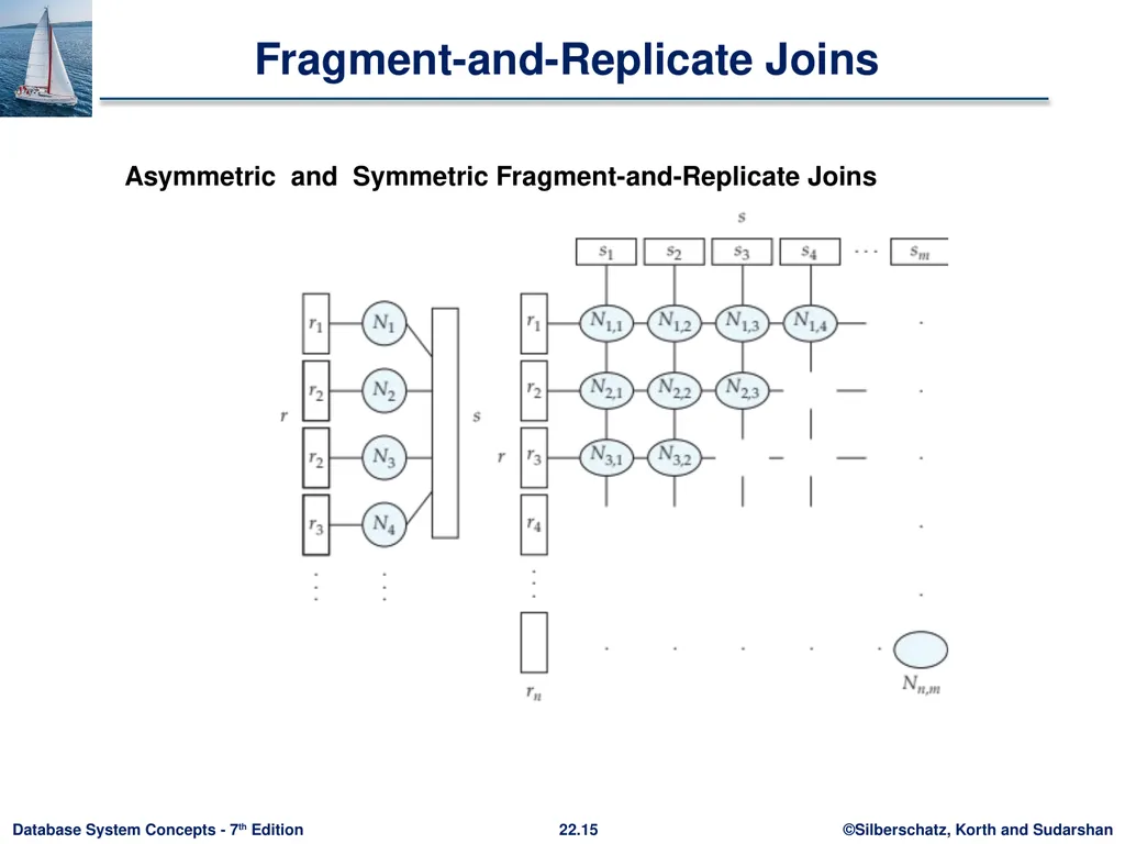
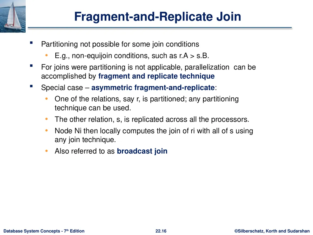
slide15. Fragment-and-Replicate Joins Asymmetric and Symmetric Fragment-and-Replicate Joins<br>
slide16. Fragment-and-Replicate Join Partitioning not possible for some join conditions
E.g., non-equijoin conditions, such as r.A > s.B.
For joins were partitioning is not applicable, parallelization can be accomplished by fragment and replicate technique
Special case – asymmetric fragment-and-replicate:
One of the relations, say r, is partitioned; any partitioning technique can be used.
The other relation, s, is replicated across all the processors.
Node Ni then locally computes the join of ri with all of s using any join technique.
Also referred to as broadcast join<br>
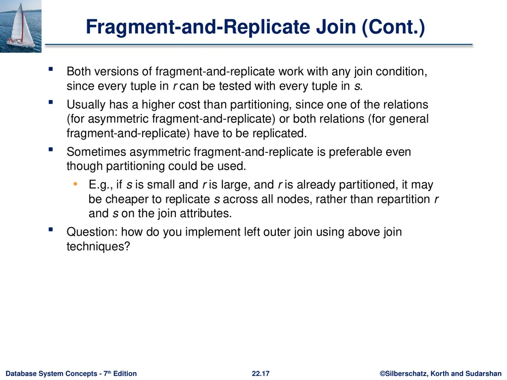
slide17. Fragment-and-Replicate Join (Cont.) Both versions of fragment-and-replicate work with any join condition, since every tuple in r can be tested with every tuple in s.
Usually has a higher cost than partitioning, since one of the relations (for asymmetric fragment-and-replicate) or both relations (for general fragment-and-replicate) have to be replicated.
Sometimes asymmetric fragment-and-replicate is preferable even though partitioning could be used.
E.g., if s is small and r is large, and r is already partitioned, it may be cheaper to replicate s across all nodes, rather than repartition r and s on the join attributes.
Question: how do you implement left outer join using above join techniques?<br>
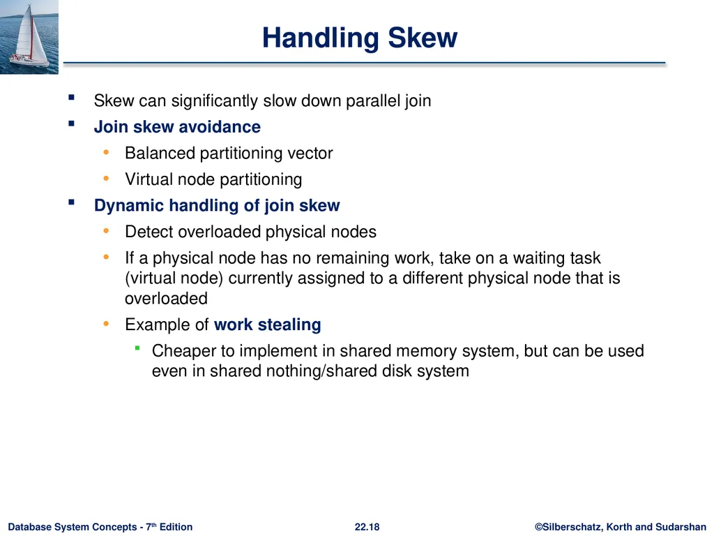
slide18. Handling Skew Skew can significantly slow down parallel join
Join skew avoidance
Balanced partitioning vector
Virtual node partitioning
Dynamic handling of join skew
Detect overloaded physical nodes
If a physical node has no remaining work, take on a waiting task (virtual node) currently assigned to a different physical node that is overloaded
Example of work stealing
Cheaper to implement in shared memory system, but can be used even in shared nothing/shared disk system<br>
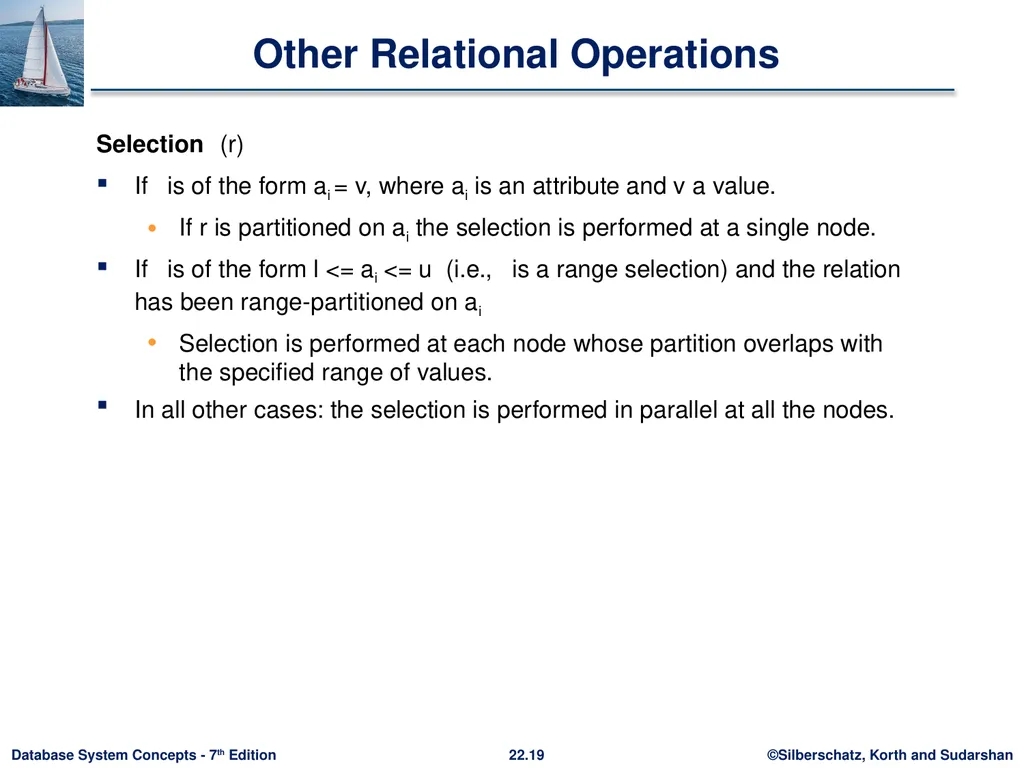
slide19. Other Relational Operations Selection (r)
If is of the form ai = v, where ai is an attribute and v a value.
If r is partitioned on ai the selection is performed at a single node.
If is of the form l <= ai <= u (i.e., is a range selection) and the relation has been range-partitioned on ai
Selection is performed at each node whose partition overlaps with the specified range of values.
In all other cases: the selection is performed in parallel at all the nodes.<br>
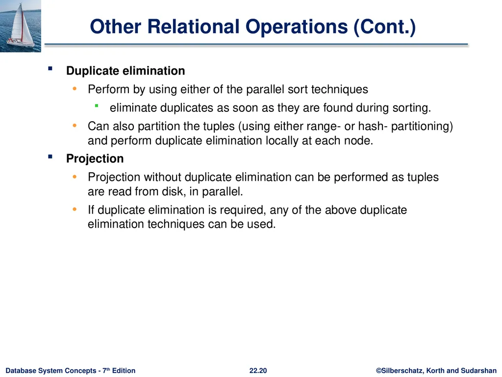
slide20. Other Relational Operations (Cont.) Duplicate elimination
Perform by using either of the parallel sort techniques
eliminate duplicates as soon as they are found during sorting.
Can also partition the tuples (using either range- or hash- partitioning) and perform duplicate elimination locally at each node.
Projection
Projection without duplicate elimination can be performed as tuples are read from disk, in parallel.
If duplicate elimination is required, any of the above duplicate elimination techniques can be used.<br>
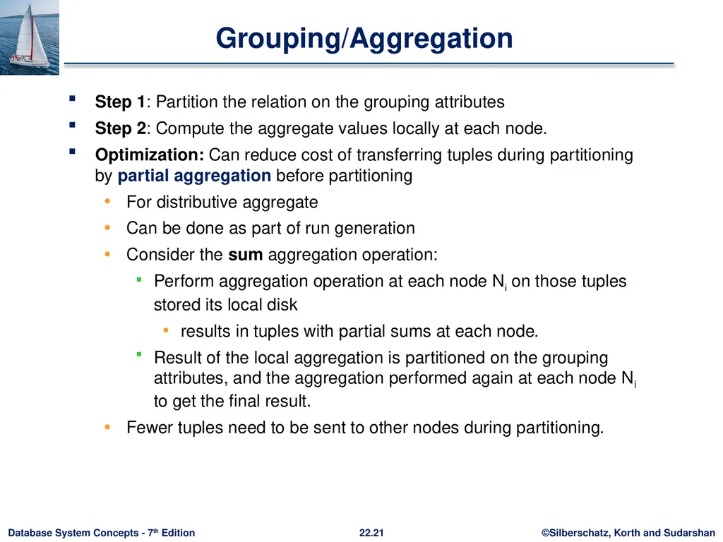
slide21. Grouping/Aggregation Step 1: Partition the relation on the grouping attributes
Step 2: Compute the aggregate values locally at each node.
Optimization: Can reduce cost of transferring tuples during partitioning by partial aggregation before partitioning
For distributive aggregate
Can be done as part of run generation
Consider the sum aggregation operation:
Perform aggregation operation at each node Ni on those tuples stored its local disk
results in tuples with partial sums at each node.
Result of the local aggregation is partitioned on the grouping attributes, and the aggregation performed again at each node Ni to get the final result.
Fewer tuples need to be sent to other nodes during partitioning.<br>
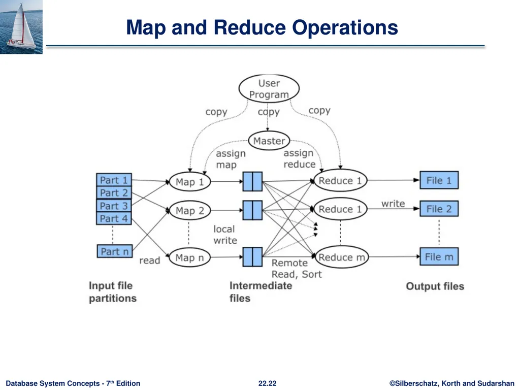
slide22. Map and Reduce Operations<br>
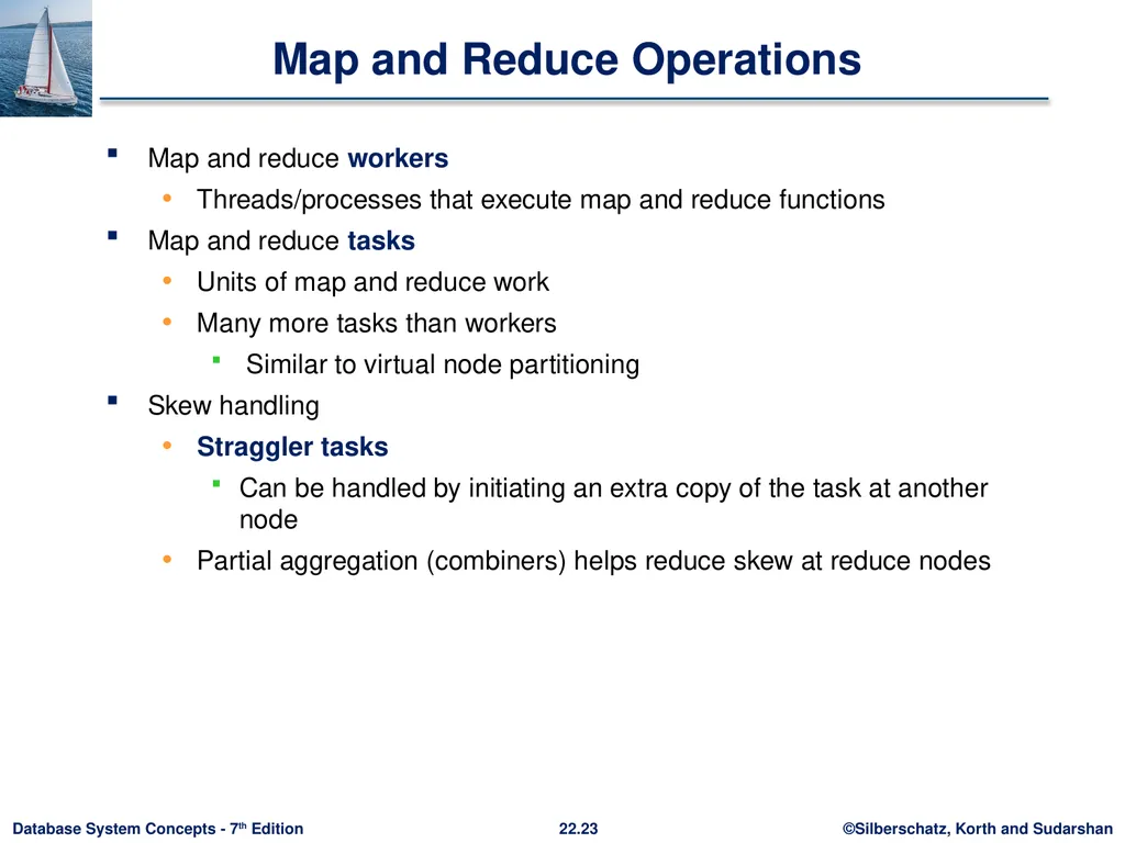
slide23. Map and Reduce Operations Map and reduce workers
Threads/processes that execute map and reduce functions
Map and reduce tasks
Units of map and reduce work
Many more tasks than workers
Similar to virtual node partitioning
Skew handling
Straggler tasks
Can be handled by initiating an extra copy of the task at another node
Partial aggregation (combiners) helps reduce skew at reduce nodes<br>
slide24. Parallel Evaluation of Query Plans<br>
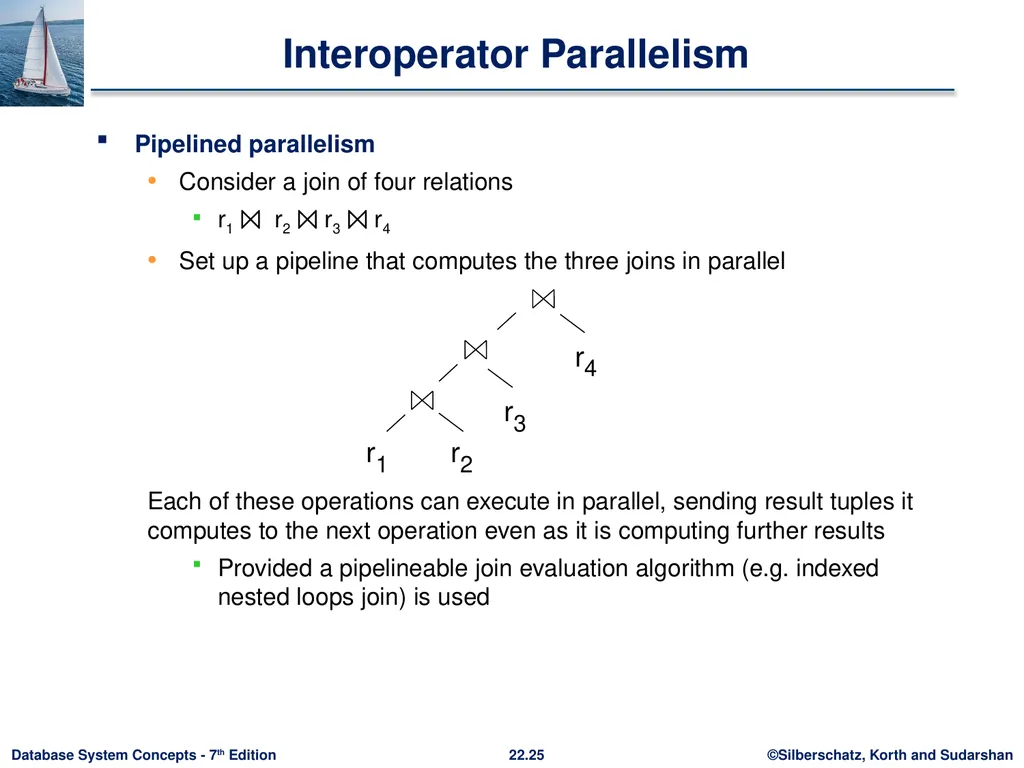
slide25. Interoperator Parallelism Pipelined parallelism
Consider a join of four relations
r1 ⨝ r2 ⨝ r3 ⨝ r4
Set up a pipeline that computes the three joins in parallel
Each of these operations can execute in parallel, sending result tuples it computes to the next operation even as it is computing further results
Provided a pipelineable join evaluation algorithm (e.g. indexed nested loops join) is used<br>
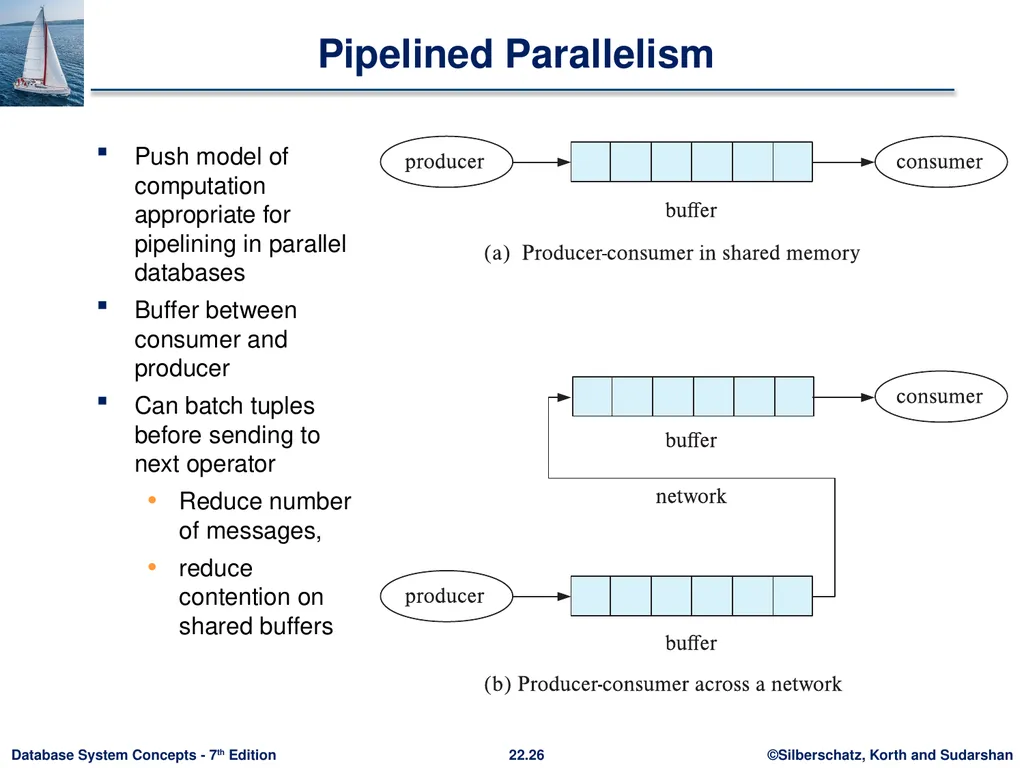
slide26. Pipelined Parallelism Push model of computation appropriate for pipelining in parallel databases
Buffer between consumer and producer
Can batch tuples before sending to next operator
Reduce number of messages,
reduce contention on shared buffers<br>
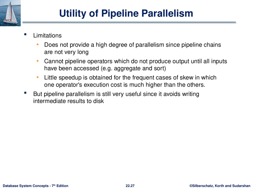
slide27. Utility of Pipeline Parallelism Limitations
Does not provide a high degree of parallelism since pipeline chains are not very long
Cannot pipeline operators which do not produce output until all inputs have been accessed (e.g. aggregate and sort)
Little speedup is obtained for the frequent cases of skew in which one operator's execution cost is much higher than the others.
But pipeline parallelism is still very useful since it avoids writing intermediate results to disk<br>
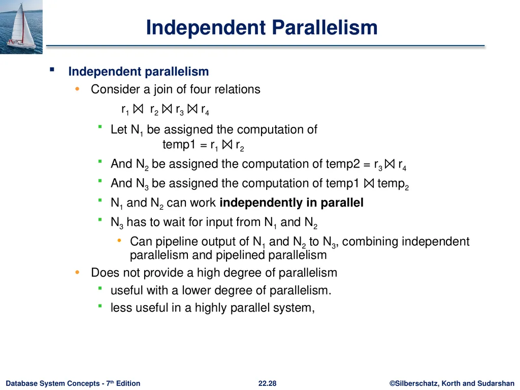
slide28. Independent Parallelism Independent parallelism
Consider a join of four relations
r1 ⨝ r2 ⨝ r3 ⨝ r4
Let N1 be assigned the computation of temp1 = r1 ⨝ r2
And N2 be assigned the computation of temp2 = r3 ⨝ r4
And N3 be assigned the computation of temp1 ⨝ temp2
N1 and N2 can work independently in parallel
N3 has to wait for input from N1 and N2
Can pipeline output of N1 and N2 to N3, combining independent parallelism and pipelined parallelism
Does not provide a high degree of parallelism
useful with a lower degree of parallelism.
less useful in a highly parallel system,<br>
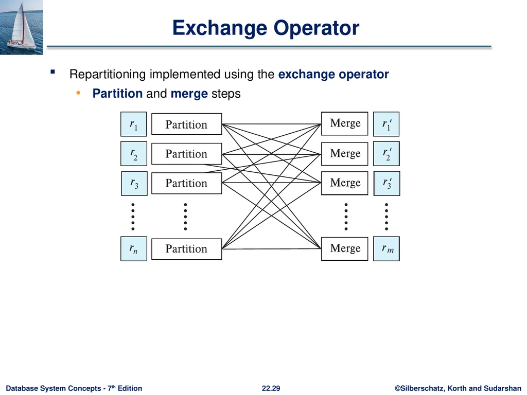
slide29. Exchange Operator Repartitioning implemented using the exchange operator
Partition and merge steps<br>
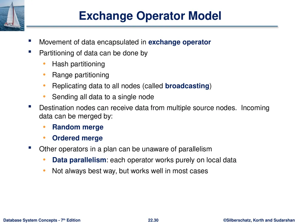
slide30. Exchange Operator Model Movement of data encapsulated in exchange operator
Partitioning of data can be done by
Hash partitioning
Range partitioning
Replicating data to all nodes (called broadcasting)
Sending all data to a single node
Destination nodes can receive data from multiple source nodes. Incoming data can be merged by:
Random merge
Ordered merge
Other operators in a plan can be unaware of parallelism
Data parallelism: each operator works purely on local data
Not always best way, but works well in most cases<br>
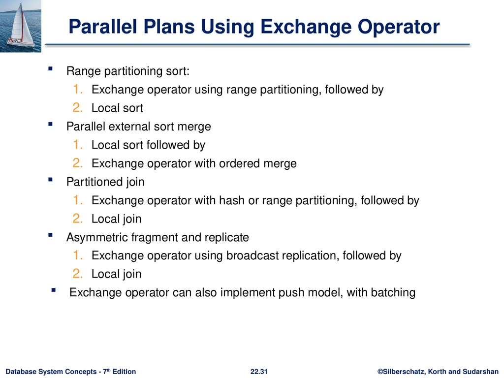
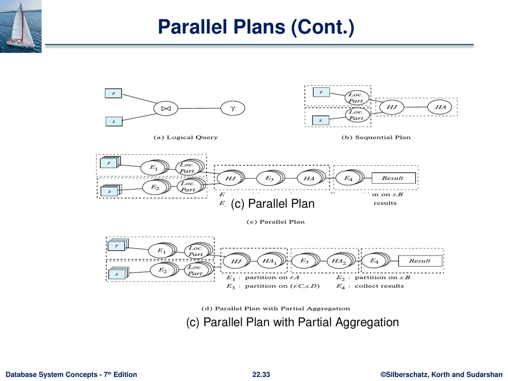
slide31. Parallel Plans Using Exchange Operator Range partitioning sort:
Exchange operator using range partitioning, followed by
Local sort
Parallel external sort merge
Local sort followed by
Exchange operator with ordered merge
Partitioned join
Exchange operator with hash or range partitioning, followed by
Local join
Asymmetric fragment and replicate
Exchange operator using broadcast replication, followed by
Local join
Exchange operator can also implement push model, with batching<br>
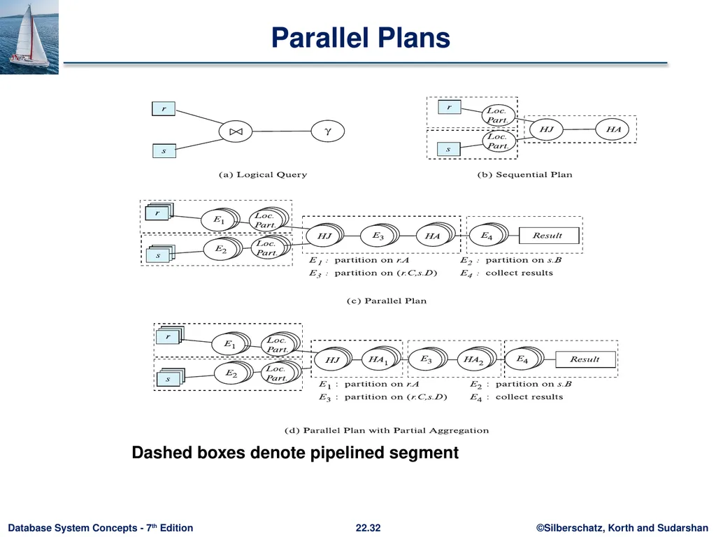
slide32. Parallel Plans Dashed boxes denote pipelined segment<br>
slide33. Parallel Plans (Cont.)<br>
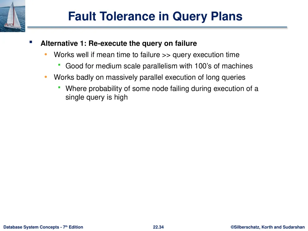
slide34. Fault Tolerance in Query Plans Alternative 1: Re-execute the query on failure
Works well if mean time to failure >> query execution time
Good for medium scale parallelism with 100’s of machines
Works badly on massively parallel execution of long queries
Where probability of some node failing during execution of a single query is high<br>
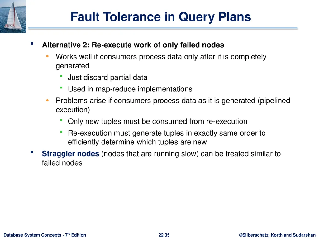
slide35. Fault Tolerance in Query Plans Alternative 2: Re-execute work of only failed nodes
Works well if consumers process data only after it is completely generated
Just discard partial data
Used in map-reduce implementations
Problems arise if consumers process data as it is generated (pipelined execution)
Only new tuples must be consumed from re-execution
Re-execution must generate tuples in exactly same order to efficiently determine which tuples are new
Straggler nodes (nodes that are running slow) can be treated similar to failed nodes<br>
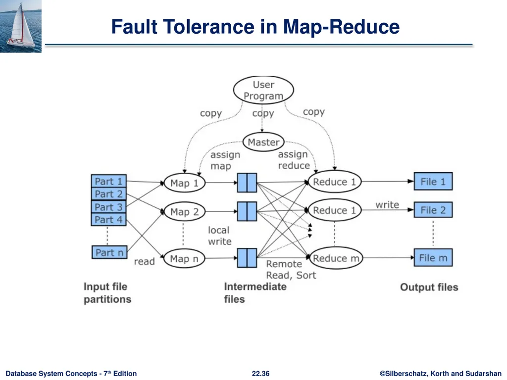
slide36. Fault Tolerance in Map-Reduce<br>
slide37. Fault Tolerance in Map Reduce Implementation Map workers writes data to local disk
Cheaper than writing to distributed file system
When task is complete, data is sent to reducers
Reducers use data only after it is fully received
On map worker failure:
Reexecute map tasks on a new node
Reducers get data from new node, discarding partially received data (if any) from failed node
On reduce worker failure
Reexecute reduce task on new node
Re-fetch data from map nodes
On completion of a map-reduce phase, result is written to distributed file system
Replication ensures result is safe from failures<br>
slide38. Fault Tolerant Query Execution Overheads of fault-tolerant query execution
Materialization cost
Each step has to wait till the previous step finishes
Stragglers can cause significant delays
Pipelined execution can avoid these costs
But harder to make pipelined execution fault-tolerant
E.g. duplication of tuples when failed task is reexecuted
Apache Spark uses concept of Resilient Distributed Datasets (RDDs)
Data can be replicated in memory/on disk
But intermediate results are not materialized
Query nodes can be reexecuted to regenerate results<br>
slide39. Query Processing in Shared Memory Systems Parallel query processing techniques discussed so far can be optimized if data is in shared memory
Shared memory parallel processing usually based on threads, instead of processes
Usually number of threads = number of cores * number off hardware threads per core<br>
slide40. Query Processing in Shared Memory Systems Optimized algorithms for shared memory
With asymmetric fragment-and-replicate join, the smaller relation can be in shared memory, instead of being replicated for each thread
Hash join can be done by
Partitioning build relation to each thread, OR
Shared build relation with singe index, in shared memory
Probe relation can be partitioned into small pieces (a.k.a. morsels)
Each thread processes one piece of the probe at a time, in parallel with other threads
Shared index construction can be parallelized, but carefully
Multiple threads may try to write to same location in shared memory
Atomic instruction (test-and-set/compare-and-swap) can be used to add entries to hash table list<br>
slide41. Query Processing in Shared Memory Systems Skew can be handled by work stealing
Idle processors can take up tasks allocated to other processors
Virtual node partitioning allows tasks to be broken into small pieces
Cost of reallocating a partition is low in shared memory
Even simpler if shared build relation is used
only probe relation partitioned need to be reassigned
Query processing algorithms should be are of NUMA: Non-uniform memory access
Each thread scheduled as far as possible on same core every time it runs
Data structures used by only 1 thread allocated in memory local to the core on which the thread is running<br>
slide42. Query Processing in Shared Memory Systems Cache-conscious algorithms used in main-memory centralized query processing should also be used in shared-memory systems
Single Instruction Multiple Data (SIMD) parallelism is increasingly used
In GPUs as well as Intel Xeon Phi co-processors
Vector processing
Vector processing can be used for relational operations<br>
slide43. Query Optimization for Parallel Query Execution<br>
slide44. Query Optimization For Parallel Execution Query optimization in parallel databases is significantly more complex than query optimization in sequential databases.
Different options for partitioning inputs and intermediate results
Cost models are more complicated, since we must take into account partitioning costs and issues such as skew and resource contention.<br>
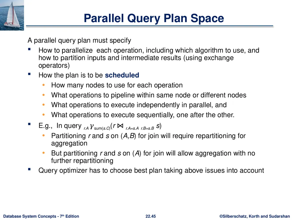
slide45. Parallel Query Plan Space A parallel query plan must specify
How to parallelize each operation, including which algorithm to use, and how to partition inputs and intermediate results (using exchange operators)
How the plan is to be scheduled
How many nodes to use for each operation
What operations to pipeline within same node or different nodes
What operations to execute independently in parallel, and
What operations to execute sequentially, one after the other.
E.g., In query r.A 𝛾sum(s.C)(r ⋈ r.A=s.A r.B=s.B s)
Partitioning r and s on (A,B) for join will require repartitioning for aggregation
But partitioning r and s on (A) for join will allow aggregation with no further repartitioning
Query optimizer has to choose best plan taking above issues into account<br>
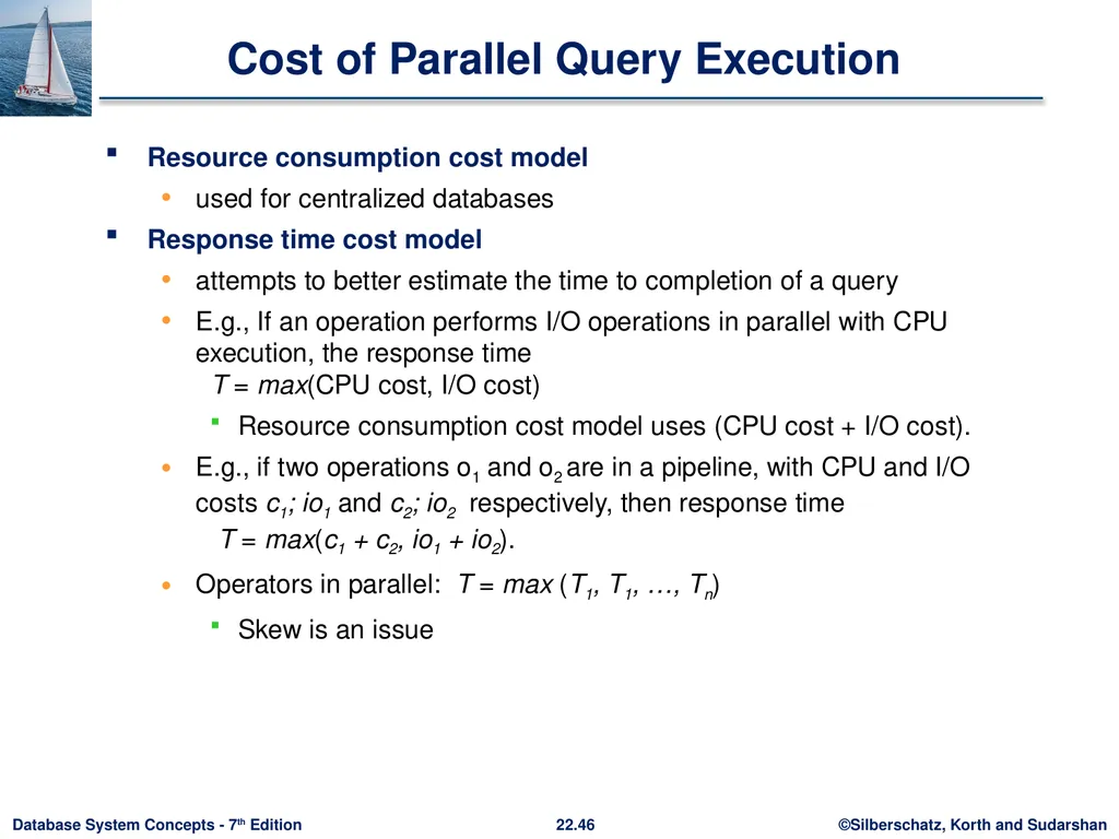
slide46. Cost of Parallel Query Execution Resource consumption cost model
used for centralized databases
Response time cost model
attempts to better estimate the time to completion of a query
E.g., If an operation performs I/O operations in parallel with CPU execution, the response time T = max(CPU cost, I/O cost)
Resource consumption cost model uses (CPU cost + I/O cost).
E.g., if two operations o1 and o2 are in a pipeline, with CPU and I/O costs c1; io1 and c2; io2 respectively, then response time T = max(c1 + c2, io1 + io2).
Operators in parallel: T = max (T1, T1, …, Tn)
Skew is an issue<br>
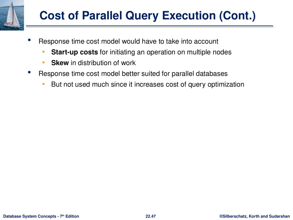
slide47. Cost of Parallel Query Execution (Cont.) Response time cost model would have to take into account
Start-up costs for initiating an operation on multiple nodes
Skew in distribution of work
Response time cost model better suited for parallel databases
But not used much since it increases cost of query optimization<br>
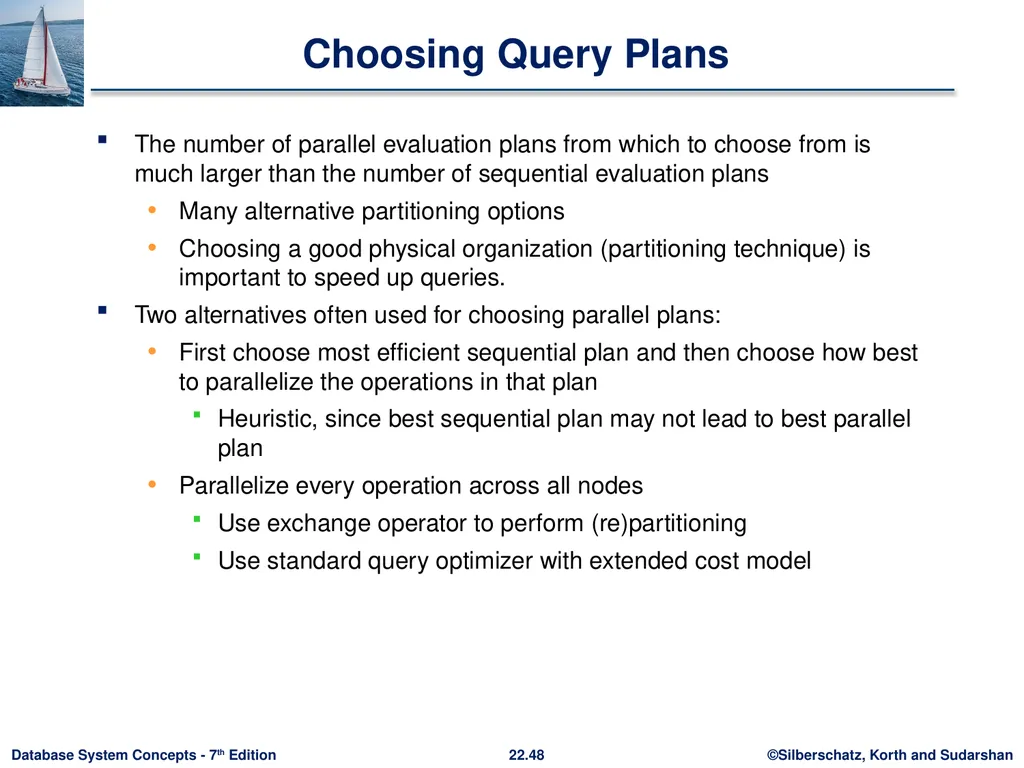
slide48. Choosing Query Plans The number of parallel evaluation plans from which to choose from is much larger than the number of sequential evaluation plans
Many alternative partitioning options
Choosing a good physical organization (partitioning technique) is important to speed up queries.
Two alternatives often used for choosing parallel plans:
First choose most efficient sequential plan and then choose how best to parallelize the operations in that plan
Heuristic, since best sequential plan may not lead to best parallel plan
Parallelize every operation across all nodes
Use exchange operator to perform (re)partitioning
Use standard query optimizer with extended cost model<br>
slide49. Physical Schema Partitioning scheme important for queries
Colocate data that is accessed together
E.g., all records for a particular user
E.g., student record with all takes records of the student
Store multiple copies of a relation, partitioned on different attributes
E.g., extra copy of takes partitioned on (course id, year, semester, sec id) for colocation with section record
Materialized views to avoid joins at query time
Materialized view itself is stored partitioned across nodes
Speeds up queries, but extra cost for updates
Extra copy of materialized view may be stored partitioned on different attributes
See book for details of parallel maintenance of materialized views<br>
slide50. Streaming Data<br>
slide51. Streaming Data Real-time analytics is increasingly important
Online processing of incoming data
But data must also be stored for later processing
Architecture alternatives:
Lambda architecture: sends a copy of data to real time stream analytics system, and another copy to data storage system
Increasingly, same system provides storage and real time stream analytics<br>
slide52. Logical Routing of Streams<br>
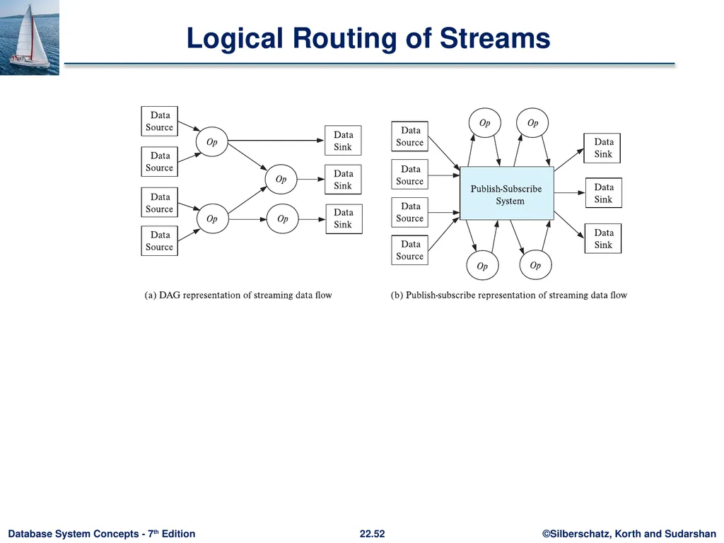
slide53. Parallel Processing of Streaming Data Logical routing of tuples is done by creating a Directed Acyclic Graph (DAG)
Can be done by creating a configuration file
Called a topology in the Apache Storm system
OR, can be done dynamically by using publish-subscribe system
E.g., Apache Kafka
Producers publish to topic/stream, consumers subscribe to topic/streams<br>
slide54. Parallel Processing of Streaming Data Physical DAG reflects parallel execution of operator instances
Parallel implementation of publish-subscribe system
Each topic/stream is partitioned (topic-partition)
Multiple instances of each operator, running in parallel
Each subscribes to one or more partitions of a topic
In Kafka, multiple instances of an operator register with an associated consumer group
Each topic-partition sent to a single consumer from the consumer group
Streaming operators often need to store state
Can be stored locally (cheaper) or in a parallel data-store (better for fault tolerance)<br>
slide55. Fault Tolerance Possible semantics when dealing with failures
At-least once
At-most once
Exactly once
Can be implemented in the publish-subscribe/routing system
Need to store tuples, including intermediate results, persistently
Can lower overhead by checkpointing operator state, and replaying operator from checkpoint, instead of persisting operator output
But need to ensure duplicates are removed
Replication of operators: Copy of operator running concurrently with original
Similar to hot-spare
Allows instant recovery from failure<br>
slide56. Distributed Query Processing<br>
slide57. Data Integration From Multiple Sources Many database applications require data from multiple databases
A federated database system is a software layer on top of existing database systems, which is designed to manipulate information in heterogeneous databases
Creates an illusion of logical database integration without any physical database integration
Each database has its local schema
Global schema integrates all the local schema
Schema integration
Queries can be issued against global schema, and translated to queries on local schemas
Databases that support common schema and queries, but not updates, are referred to as mediator systems<br>
slide58. Data Integration From Multiple Sources Data virtualization
Allows data access from multiple databases, but without a common schema
External data approach: allows database to treat external data as a database relation (foreign tables)
Many databases today allow a local table to be defined as a view on external data
SQL Management of External Data (SQL MED) standard
Wrapper for a data source is a view that translates data from local to a global schema
Wrappers must also translate updates on global schema to updates on local schema<br>
slide59. Data Warehouses and Data Lakes Data warehouse is an alternative to data integration
Migrates data to a common schema, avoiding run-time overhead
Cost of translating schema/data to a common warehouse schema can be significant
Data lake: architecture where data is stored in multiple data storage systems, in different storage formats, but which can be queried from a single system.<br>
slide60. Schema and Data Integration Schema integration: creating a unified conceptual schema
Requires creation of global schema, integrating a number of local schema
Global-as-view approach
At each site, create a view of local data, mapping it to the global schema
Union of local views is the global view
Good for queries, but not for updates
E.g., which local database should an insert go to?
Local-as-view approach
Create a view defining contents of local data as a view of global data
Site stores local data as before, the view is for update processing
Updates on global schema are mapped to updates to the local views
See book for more details with an example<br>
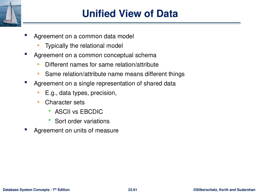
slide61. Unified View of Data Agreement on a common data model
Typically the relational model
Agreement on a common conceptual schema
Different names for same relation/attribute
Same relation/attribute name means different things
Agreement on a single representation of shared data
E.g., data types, precision,
Character sets
ASCII vs EBCDIC
Sort order variations
Agreement on units of measure<br>
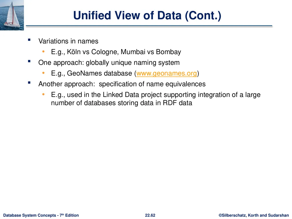
slide62. Unified View of Data (Cont.) Variations in names
E.g., Köln vs Cologne, Mumbai vs Bombay
One approach: globally unique naming system
E.g., GeoNames database (www.geonames.org)
Another approach: specification of name equivalences
E.g., used in the Linked Data project supporting integration of a large number of databases storing data in RDF data<br>
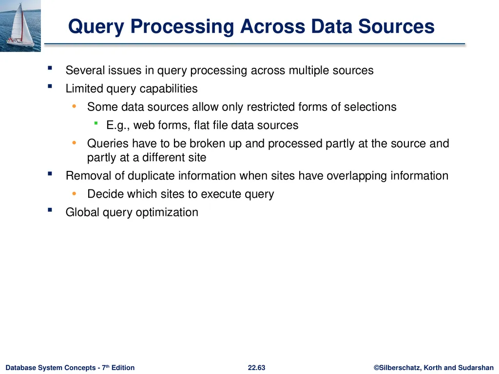
slide63. Query Processing Across Data Sources Several issues in query processing across multiple sources
Limited query capabilities
Some data sources allow only restricted forms of selections
E.g., web forms, flat file data sources
Queries have to be broken up and processed partly at the source and partly at a different site
Removal of duplicate information when sites have overlapping information
Decide which sites to execute query
Global query optimization<br>
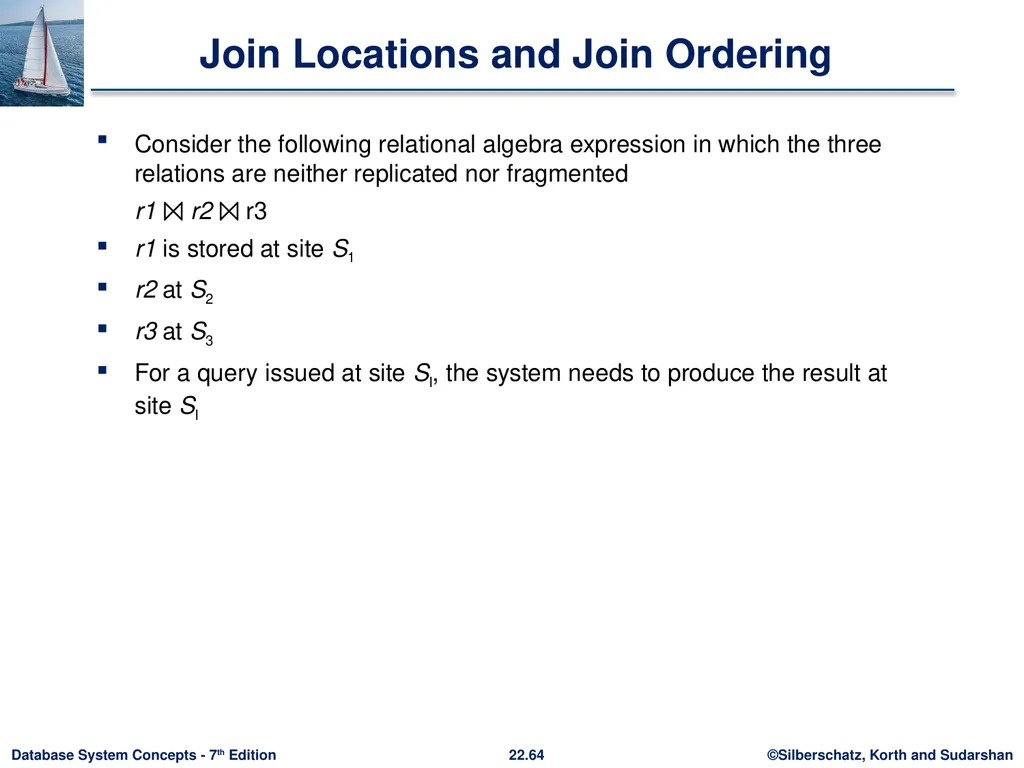
slide64. Join Locations and Join Ordering Consider the following relational algebra expression in which the three relations are neither replicated nor fragmented
r1 ⨝ r2 ⨝ r3
r1 is stored at site S1
r2 at S2
r3 at S3
For a query issued at site SI, the system needs to produce the result at site SI<br>
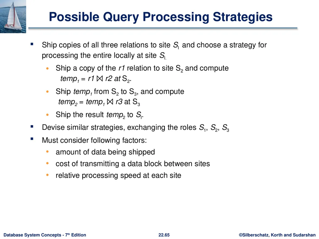
slide65. Possible Query Processing Strategies Ship copies of all three relations to site SI and choose a strategy for processing the entire locally at site SI.
Ship a copy of the r1 relation to site S2 and compute temp1 = r1 ⨝ r2 at S2.
Ship temp1 from S2 to S3, and compute temp2 = temp1 ⨝ r3 at S3
Ship the result temp2 to SI.
Devise similar strategies, exchanging the roles S1, S2, S3
Must consider following factors:
amount of data being shipped
cost of transmitting a data block between sites
relative processing speed at each site<br>
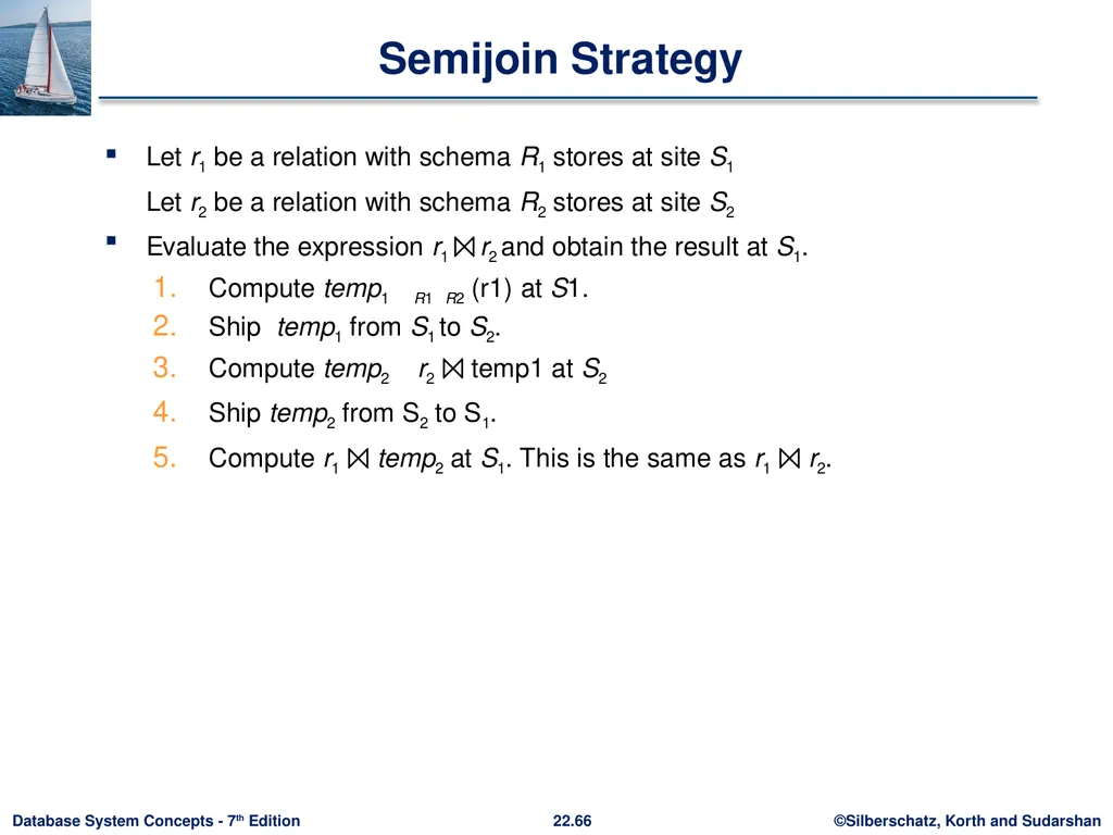
slide66. Semijoin Strategy Let r1 be a relation with schema R1 stores at site S1
Let r2 be a relation with schema R2 stores at site S2
Evaluate the expression r1 ⨝ r2 and obtain the result at S1.
Compute temp1 R1 R2 (r1) at S1.
Ship temp1 from S1 to S2.
Compute temp2 r2 ⨝ temp1 at S2
Ship temp2 from S2 to S1.
Compute r1 ⨝ temp2 at S1. This is the same as r1 ⨝ r2.<br>
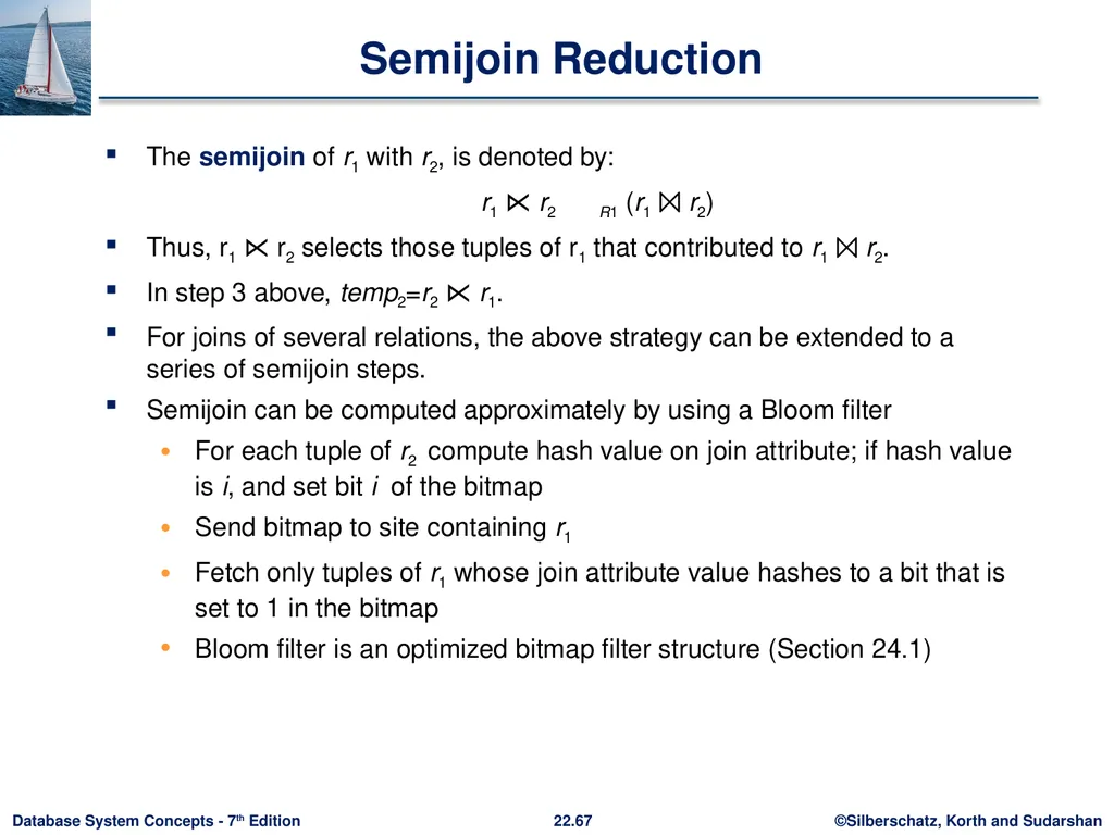
slide67. Semijoin Reduction The semijoin of r1 with r2, is denoted by:
r1 ⋉ r2 R1 (r1 ⨝ r2)
Thus, r1 ⋉ r2 selects those tuples of r1 that contributed to r1 ⨝ r2.
In step 3 above, temp2=r2 ⋉ r1.
For joins of several relations, the above strategy can be extended to a series of semijoin steps.
Semijoin can be computed approximately by using a Bloom filter
For each tuple of r2 compute hash value on join attribute; if hash value is i, and set bit i of the bitmap
Send bitmap to site containing r1
Fetch only tuples of r1 whose join attribute value hashes to a bit that is set to 1 in the bitmap
Bloom filter is an optimized bitmap filter structure (Section 24.1)<br>
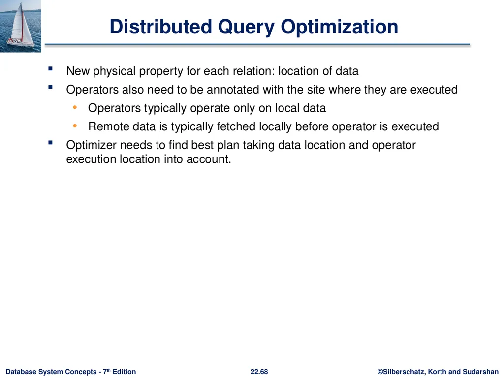
slide68. Distributed Query Optimization New physical property for each relation: location of data
Operators also need to be annotated with the site where they are executed
Operators typically operate only on local data
Remote data is typically fetched locally before operator is executed
Optimizer needs to find best plan taking data location and operator execution location into account.<br>
slide69. Distributed Directory Systems Distributed directory systems are widely used
Internet Domain Name Service (DNS)
Lightweight Directory Access Protocol (LDAP)
Widely used to store organizational data, especially user profiles
Data in a distributed directory system are stored and controlled in a distributed hierarchical manner
E.g., data about yale.edu is provided by a Yale, and about IIT Bombay by an IIT Bombay server
Data can be queries in a uniform manner regardless of where it is stored
Queries get forwarded to the site where the information is stored<br>
slide70. End of Chapter 22<br>
slide2. Chapter 22: Parallel And Distributed Query Processing Overview
Parallel Sort
Parallel Join
Other Operations
Parallel Evaluation of Query Plans
Query Processing on Shared Memory
Query Optimization
Distributed Query Processing<br>
slide3. Parallel Query Processing Different queries/transactions can be run in parallel with each other.
Interquery parallelism
Concurrency control takes care of conflicts in case of updates
More on parallel transaction processing in Chapter 23
Focus in this chapter is on read-only queries
Individual relational operations (e.g., sort, join, aggregation) can be executed in parallel
data can be partitioned and each processor can work independently on its own partition.
Queries are expressed in high level language (SQL, translated to relational algebra)
makes parallelization easier.<br>
slide4. Intraquery Parallelism Intraquery parallelism: execution of a single query in parallel on multiple processors/disks; important for speeding up long-running queries.
Two complementary forms of intraquery parallelism:
Intraoperation Parallelism – parallelize the execution of each individual operation in the query
Supports high degree of parallelism
Interoperation Parallelism – execute the different operations in a query expression in parallel.
Limited degree of parallelism<br>
slide5. Parallel Processing of Relational Operations Our discussion of parallel algorithms assumes:
read-only queries
shared-nothing architecture
n nodes, N1, ..., Nn
Each assumed to have disks and processors.
Initial focus on parallelization to a shared-nothing node
Parallel processing within a shared memory/shared disk node discussed later
Shared-nothing architectures can be efficiently simulated on shared-memory and shared-disk systems.
Algorithms for shared-nothing systems can thus be run on shared-memory and shared-disk systems.
However, some optimizations may be possible.<br>
slide6. Intraoperation Parallelism<br>
slide7. Range Partitioning<br>
slide8. Range-Partitioning Parallel Sort<br>
slide9. Parallel Sort<br>
slide10. Parallel Sort Range-Partitioning Sort
Choose nodes N1, ..., Nm, where m n -1 to do sorting.
Create range-partition vector with m-1 entries, on the sorting attributes
Redistribute the relation using range partitioning
Each node Ni sorts its partition of the relation locally.
Example of data parallelism: each node executes same operation in parallel with other nodes, without any interaction with the others.
Final merge operation is trivial: range-partitioning ensures that, if i < j, all key values in node Ni are all less than all key values in Nj.<br>
slide11. Parallel Sort (Cont.) Parallel External Sort-Merge
Assume the relation has already been partitioned among nodes N1, ..., Nn (in whatever manner).
Each node Ni locally sorts the data (using local disk as required)
The sorted runs on each node are then merged in parallel:
The sorted partitions at each node Ni are range-partitioned across the processors N1, ..., Nn.
Each node Ni performs a merge on the streams as they are received, to get a single sorted run.
The sorted runs on nodes N1, ..., Nn are concatenated to get the final result.
Algorithm as described vulnerable to execution skew
all nodes send to node 1, then all nodes send data to node 2, …
Can be modified so each node sends data to all other nodes in parallel (block at a time)<br>
slide12. Partitioned Parallel Join Partition using range or hash partitioning, on join attributes<br>
slide13. Partitioned Parallel Join (Cont.) For equi-joins and natural joins, it is possible to partition the two input relations across the processors, and compute the join locally at each processor.
Can use either range partitioning or hash partitioning.
r and s must be partitioned on their join attributes r.A and s.B), using the same range-partitioning vector or hash function.
Join can be computed at each site using any of
Hash join, leading to partitioned parallel hash join
Merge join, leading to partitioned parallel merge join
Nested loops join, leading to partitioned parallel nested-loops join or partitioned parallel index nested-loops join<br>
slide14. Partitioned Parallel Hash-Join Parallelizing partitioned hash join:
A hash function h1 takes the join attribute value of each tuple in s and maps this tuple to one of the n nodes.
As tuples of relation s are received at the destination nodes, they are partitioned further using another hash function, h2, which is used to compute the hash-join locally.
Repeat above for each tuple in r.
Each node Ni executes the build and probe phases of the hash-join algorithm on the local partitions ri and si of r and s to produce a partition of the final result of the hash-join.
Note: Hash-join optimizations can be applied to the parallel case
e.g., the hybrid hash-join algorithm can be used to cache some of the incoming tuples in memory and avoid the cost of writing them and reading them back in.<br>
slide15. Fragment-and-Replicate Joins Asymmetric and Symmetric Fragment-and-Replicate Joins<br>
slide16. Fragment-and-Replicate Join Partitioning not possible for some join conditions
E.g., non-equijoin conditions, such as r.A > s.B.
For joins were partitioning is not applicable, parallelization can be accomplished by fragment and replicate technique
Special case – asymmetric fragment-and-replicate:
One of the relations, say r, is partitioned; any partitioning technique can be used.
The other relation, s, is replicated across all the processors.
Node Ni then locally computes the join of ri with all of s using any join technique.
Also referred to as broadcast join<br>
slide17. Fragment-and-Replicate Join (Cont.) Both versions of fragment-and-replicate work with any join condition, since every tuple in r can be tested with every tuple in s.
Usually has a higher cost than partitioning, since one of the relations (for asymmetric fragment-and-replicate) or both relations (for general fragment-and-replicate) have to be replicated.
Sometimes asymmetric fragment-and-replicate is preferable even though partitioning could be used.
E.g., if s is small and r is large, and r is already partitioned, it may be cheaper to replicate s across all nodes, rather than repartition r and s on the join attributes.
Question: how do you implement left outer join using above join techniques?<br>
slide18. Handling Skew Skew can significantly slow down parallel join
Join skew avoidance
Balanced partitioning vector
Virtual node partitioning
Dynamic handling of join skew
Detect overloaded physical nodes
If a physical node has no remaining work, take on a waiting task (virtual node) currently assigned to a different physical node that is overloaded
Example of work stealing
Cheaper to implement in shared memory system, but can be used even in shared nothing/shared disk system<br>
slide19. Other Relational Operations Selection (r)
If is of the form ai = v, where ai is an attribute and v a value.
If r is partitioned on ai the selection is performed at a single node.
If is of the form l <= ai <= u (i.e., is a range selection) and the relation has been range-partitioned on ai
Selection is performed at each node whose partition overlaps with the specified range of values.
In all other cases: the selection is performed in parallel at all the nodes.<br>
slide20. Other Relational Operations (Cont.) Duplicate elimination
Perform by using either of the parallel sort techniques
eliminate duplicates as soon as they are found during sorting.
Can also partition the tuples (using either range- or hash- partitioning) and perform duplicate elimination locally at each node.
Projection
Projection without duplicate elimination can be performed as tuples are read from disk, in parallel.
If duplicate elimination is required, any of the above duplicate elimination techniques can be used.<br>
slide21. Grouping/Aggregation Step 1: Partition the relation on the grouping attributes
Step 2: Compute the aggregate values locally at each node.
Optimization: Can reduce cost of transferring tuples during partitioning by partial aggregation before partitioning
For distributive aggregate
Can be done as part of run generation
Consider the sum aggregation operation:
Perform aggregation operation at each node Ni on those tuples stored its local disk
results in tuples with partial sums at each node.
Result of the local aggregation is partitioned on the grouping attributes, and the aggregation performed again at each node Ni to get the final result.
Fewer tuples need to be sent to other nodes during partitioning.<br>
slide22. Map and Reduce Operations<br>
slide23. Map and Reduce Operations Map and reduce workers
Threads/processes that execute map and reduce functions
Map and reduce tasks
Units of map and reduce work
Many more tasks than workers
Similar to virtual node partitioning
Skew handling
Straggler tasks
Can be handled by initiating an extra copy of the task at another node
Partial aggregation (combiners) helps reduce skew at reduce nodes<br>
slide24. Parallel Evaluation of Query Plans<br>
slide25. Interoperator Parallelism Pipelined parallelism
Consider a join of four relations
r1 ⨝ r2 ⨝ r3 ⨝ r4
Set up a pipeline that computes the three joins in parallel
Each of these operations can execute in parallel, sending result tuples it computes to the next operation even as it is computing further results
Provided a pipelineable join evaluation algorithm (e.g. indexed nested loops join) is used<br>
slide26. Pipelined Parallelism Push model of computation appropriate for pipelining in parallel databases
Buffer between consumer and producer
Can batch tuples before sending to next operator
Reduce number of messages,
reduce contention on shared buffers<br>
slide27. Utility of Pipeline Parallelism Limitations
Does not provide a high degree of parallelism since pipeline chains are not very long
Cannot pipeline operators which do not produce output until all inputs have been accessed (e.g. aggregate and sort)
Little speedup is obtained for the frequent cases of skew in which one operator's execution cost is much higher than the others.
But pipeline parallelism is still very useful since it avoids writing intermediate results to disk<br>
slide28. Independent Parallelism Independent parallelism
Consider a join of four relations
r1 ⨝ r2 ⨝ r3 ⨝ r4
Let N1 be assigned the computation of temp1 = r1 ⨝ r2
And N2 be assigned the computation of temp2 = r3 ⨝ r4
And N3 be assigned the computation of temp1 ⨝ temp2
N1 and N2 can work independently in parallel
N3 has to wait for input from N1 and N2
Can pipeline output of N1 and N2 to N3, combining independent parallelism and pipelined parallelism
Does not provide a high degree of parallelism
useful with a lower degree of parallelism.
less useful in a highly parallel system,<br>
slide29. Exchange Operator Repartitioning implemented using the exchange operator
Partition and merge steps<br>
slide30. Exchange Operator Model Movement of data encapsulated in exchange operator
Partitioning of data can be done by
Hash partitioning
Range partitioning
Replicating data to all nodes (called broadcasting)
Sending all data to a single node
Destination nodes can receive data from multiple source nodes. Incoming data can be merged by:
Random merge
Ordered merge
Other operators in a plan can be unaware of parallelism
Data parallelism: each operator works purely on local data
Not always best way, but works well in most cases<br>
slide31. Parallel Plans Using Exchange Operator Range partitioning sort:
Exchange operator using range partitioning, followed by
Local sort
Parallel external sort merge
Local sort followed by
Exchange operator with ordered merge
Partitioned join
Exchange operator with hash or range partitioning, followed by
Local join
Asymmetric fragment and replicate
Exchange operator using broadcast replication, followed by
Local join
Exchange operator can also implement push model, with batching<br>
slide32. Parallel Plans Dashed boxes denote pipelined segment<br>
slide33. Parallel Plans (Cont.)<br>
slide34. Fault Tolerance in Query Plans Alternative 1: Re-execute the query on failure
Works well if mean time to failure >> query execution time
Good for medium scale parallelism with 100’s of machines
Works badly on massively parallel execution of long queries
Where probability of some node failing during execution of a single query is high<br>
slide35. Fault Tolerance in Query Plans Alternative 2: Re-execute work of only failed nodes
Works well if consumers process data only after it is completely generated
Just discard partial data
Used in map-reduce implementations
Problems arise if consumers process data as it is generated (pipelined execution)
Only new tuples must be consumed from re-execution
Re-execution must generate tuples in exactly same order to efficiently determine which tuples are new
Straggler nodes (nodes that are running slow) can be treated similar to failed nodes<br>
slide36. Fault Tolerance in Map-Reduce<br>
slide37. Fault Tolerance in Map Reduce Implementation Map workers writes data to local disk
Cheaper than writing to distributed file system
When task is complete, data is sent to reducers
Reducers use data only after it is fully received
On map worker failure:
Reexecute map tasks on a new node
Reducers get data from new node, discarding partially received data (if any) from failed node
On reduce worker failure
Reexecute reduce task on new node
Re-fetch data from map nodes
On completion of a map-reduce phase, result is written to distributed file system
Replication ensures result is safe from failures<br>
slide38. Fault Tolerant Query Execution Overheads of fault-tolerant query execution
Materialization cost
Each step has to wait till the previous step finishes
Stragglers can cause significant delays
Pipelined execution can avoid these costs
But harder to make pipelined execution fault-tolerant
E.g. duplication of tuples when failed task is reexecuted
Apache Spark uses concept of Resilient Distributed Datasets (RDDs)
Data can be replicated in memory/on disk
But intermediate results are not materialized
Query nodes can be reexecuted to regenerate results<br>
slide39. Query Processing in Shared Memory Systems Parallel query processing techniques discussed so far can be optimized if data is in shared memory
Shared memory parallel processing usually based on threads, instead of processes
Usually number of threads = number of cores * number off hardware threads per core<br>
slide40. Query Processing in Shared Memory Systems Optimized algorithms for shared memory
With asymmetric fragment-and-replicate join, the smaller relation can be in shared memory, instead of being replicated for each thread
Hash join can be done by
Partitioning build relation to each thread, OR
Shared build relation with singe index, in shared memory
Probe relation can be partitioned into small pieces (a.k.a. morsels)
Each thread processes one piece of the probe at a time, in parallel with other threads
Shared index construction can be parallelized, but carefully
Multiple threads may try to write to same location in shared memory
Atomic instruction (test-and-set/compare-and-swap) can be used to add entries to hash table list<br>
slide41. Query Processing in Shared Memory Systems Skew can be handled by work stealing
Idle processors can take up tasks allocated to other processors
Virtual node partitioning allows tasks to be broken into small pieces
Cost of reallocating a partition is low in shared memory
Even simpler if shared build relation is used
only probe relation partitioned need to be reassigned
Query processing algorithms should be are of NUMA: Non-uniform memory access
Each thread scheduled as far as possible on same core every time it runs
Data structures used by only 1 thread allocated in memory local to the core on which the thread is running<br>
slide42. Query Processing in Shared Memory Systems Cache-conscious algorithms used in main-memory centralized query processing should also be used in shared-memory systems
Single Instruction Multiple Data (SIMD) parallelism is increasingly used
In GPUs as well as Intel Xeon Phi co-processors
Vector processing
Vector processing can be used for relational operations<br>
slide43. Query Optimization for Parallel Query Execution<br>
slide44. Query Optimization For Parallel Execution Query optimization in parallel databases is significantly more complex than query optimization in sequential databases.
Different options for partitioning inputs and intermediate results
Cost models are more complicated, since we must take into account partitioning costs and issues such as skew and resource contention.<br>
slide45. Parallel Query Plan Space A parallel query plan must specify
How to parallelize each operation, including which algorithm to use, and how to partition inputs and intermediate results (using exchange operators)
How the plan is to be scheduled
How many nodes to use for each operation
What operations to pipeline within same node or different nodes
What operations to execute independently in parallel, and
What operations to execute sequentially, one after the other.
E.g., In query r.A 𝛾sum(s.C)(r ⋈ r.A=s.A r.B=s.B s)
Partitioning r and s on (A,B) for join will require repartitioning for aggregation
But partitioning r and s on (A) for join will allow aggregation with no further repartitioning
Query optimizer has to choose best plan taking above issues into account<br>
slide46. Cost of Parallel Query Execution Resource consumption cost model
used for centralized databases
Response time cost model
attempts to better estimate the time to completion of a query
E.g., If an operation performs I/O operations in parallel with CPU execution, the response time T = max(CPU cost, I/O cost)
Resource consumption cost model uses (CPU cost + I/O cost).
E.g., if two operations o1 and o2 are in a pipeline, with CPU and I/O costs c1; io1 and c2; io2 respectively, then response time T = max(c1 + c2, io1 + io2).
Operators in parallel: T = max (T1, T1, …, Tn)
Skew is an issue<br>
slide47. Cost of Parallel Query Execution (Cont.) Response time cost model would have to take into account
Start-up costs for initiating an operation on multiple nodes
Skew in distribution of work
Response time cost model better suited for parallel databases
But not used much since it increases cost of query optimization<br>
slide48. Choosing Query Plans The number of parallel evaluation plans from which to choose from is much larger than the number of sequential evaluation plans
Many alternative partitioning options
Choosing a good physical organization (partitioning technique) is important to speed up queries.
Two alternatives often used for choosing parallel plans:
First choose most efficient sequential plan and then choose how best to parallelize the operations in that plan
Heuristic, since best sequential plan may not lead to best parallel plan
Parallelize every operation across all nodes
Use exchange operator to perform (re)partitioning
Use standard query optimizer with extended cost model<br>
slide49. Physical Schema Partitioning scheme important for queries
Colocate data that is accessed together
E.g., all records for a particular user
E.g., student record with all takes records of the student
Store multiple copies of a relation, partitioned on different attributes
E.g., extra copy of takes partitioned on (course id, year, semester, sec id) for colocation with section record
Materialized views to avoid joins at query time
Materialized view itself is stored partitioned across nodes
Speeds up queries, but extra cost for updates
Extra copy of materialized view may be stored partitioned on different attributes
See book for details of parallel maintenance of materialized views<br>
slide50. Streaming Data<br>
slide51. Streaming Data Real-time analytics is increasingly important
Online processing of incoming data
But data must also be stored for later processing
Architecture alternatives:
Lambda architecture: sends a copy of data to real time stream analytics system, and another copy to data storage system
Increasingly, same system provides storage and real time stream analytics<br>
slide52. Logical Routing of Streams<br>
slide53. Parallel Processing of Streaming Data Logical routing of tuples is done by creating a Directed Acyclic Graph (DAG)
Can be done by creating a configuration file
Called a topology in the Apache Storm system
OR, can be done dynamically by using publish-subscribe system
E.g., Apache Kafka
Producers publish to topic/stream, consumers subscribe to topic/streams<br>
slide54. Parallel Processing of Streaming Data Physical DAG reflects parallel execution of operator instances
Parallel implementation of publish-subscribe system
Each topic/stream is partitioned (topic-partition)
Multiple instances of each operator, running in parallel
Each subscribes to one or more partitions of a topic
In Kafka, multiple instances of an operator register with an associated consumer group
Each topic-partition sent to a single consumer from the consumer group
Streaming operators often need to store state
Can be stored locally (cheaper) or in a parallel data-store (better for fault tolerance)<br>
slide55. Fault Tolerance Possible semantics when dealing with failures
At-least once
At-most once
Exactly once
Can be implemented in the publish-subscribe/routing system
Need to store tuples, including intermediate results, persistently
Can lower overhead by checkpointing operator state, and replaying operator from checkpoint, instead of persisting operator output
But need to ensure duplicates are removed
Replication of operators: Copy of operator running concurrently with original
Similar to hot-spare
Allows instant recovery from failure<br>
slide56. Distributed Query Processing<br>
slide57. Data Integration From Multiple Sources Many database applications require data from multiple databases
A federated database system is a software layer on top of existing database systems, which is designed to manipulate information in heterogeneous databases
Creates an illusion of logical database integration without any physical database integration
Each database has its local schema
Global schema integrates all the local schema
Schema integration
Queries can be issued against global schema, and translated to queries on local schemas
Databases that support common schema and queries, but not updates, are referred to as mediator systems<br>
slide58. Data Integration From Multiple Sources Data virtualization
Allows data access from multiple databases, but without a common schema
External data approach: allows database to treat external data as a database relation (foreign tables)
Many databases today allow a local table to be defined as a view on external data
SQL Management of External Data (SQL MED) standard
Wrapper for a data source is a view that translates data from local to a global schema
Wrappers must also translate updates on global schema to updates on local schema<br>
slide59. Data Warehouses and Data Lakes Data warehouse is an alternative to data integration
Migrates data to a common schema, avoiding run-time overhead
Cost of translating schema/data to a common warehouse schema can be significant
Data lake: architecture where data is stored in multiple data storage systems, in different storage formats, but which can be queried from a single system.<br>
slide60. Schema and Data Integration Schema integration: creating a unified conceptual schema
Requires creation of global schema, integrating a number of local schema
Global-as-view approach
At each site, create a view of local data, mapping it to the global schema
Union of local views is the global view
Good for queries, but not for updates
E.g., which local database should an insert go to?
Local-as-view approach
Create a view defining contents of local data as a view of global data
Site stores local data as before, the view is for update processing
Updates on global schema are mapped to updates to the local views
See book for more details with an example<br>
slide61. Unified View of Data Agreement on a common data model
Typically the relational model
Agreement on a common conceptual schema
Different names for same relation/attribute
Same relation/attribute name means different things
Agreement on a single representation of shared data
E.g., data types, precision,
Character sets
ASCII vs EBCDIC
Sort order variations
Agreement on units of measure<br>
slide62. Unified View of Data (Cont.) Variations in names
E.g., Köln vs Cologne, Mumbai vs Bombay
One approach: globally unique naming system
E.g., GeoNames database (www.geonames.org)
Another approach: specification of name equivalences
E.g., used in the Linked Data project supporting integration of a large number of databases storing data in RDF data<br>
slide63. Query Processing Across Data Sources Several issues in query processing across multiple sources
Limited query capabilities
Some data sources allow only restricted forms of selections
E.g., web forms, flat file data sources
Queries have to be broken up and processed partly at the source and partly at a different site
Removal of duplicate information when sites have overlapping information
Decide which sites to execute query
Global query optimization<br>
slide64. Join Locations and Join Ordering Consider the following relational algebra expression in which the three relations are neither replicated nor fragmented
r1 ⨝ r2 ⨝ r3
r1 is stored at site S1
r2 at S2
r3 at S3
For a query issued at site SI, the system needs to produce the result at site SI<br>
slide65. Possible Query Processing Strategies Ship copies of all three relations to site SI and choose a strategy for processing the entire locally at site SI.
Ship a copy of the r1 relation to site S2 and compute temp1 = r1 ⨝ r2 at S2.
Ship temp1 from S2 to S3, and compute temp2 = temp1 ⨝ r3 at S3
Ship the result temp2 to SI.
Devise similar strategies, exchanging the roles S1, S2, S3
Must consider following factors:
amount of data being shipped
cost of transmitting a data block between sites
relative processing speed at each site<br>
slide66. Semijoin Strategy Let r1 be a relation with schema R1 stores at site S1
Let r2 be a relation with schema R2 stores at site S2
Evaluate the expression r1 ⨝ r2 and obtain the result at S1.
Compute temp1 R1 R2 (r1) at S1.
Ship temp1 from S1 to S2.
Compute temp2 r2 ⨝ temp1 at S2
Ship temp2 from S2 to S1.
Compute r1 ⨝ temp2 at S1. This is the same as r1 ⨝ r2.<br>
slide67. Semijoin Reduction The semijoin of r1 with r2, is denoted by:
r1 ⋉ r2 R1 (r1 ⨝ r2)
Thus, r1 ⋉ r2 selects those tuples of r1 that contributed to r1 ⨝ r2.
In step 3 above, temp2=r2 ⋉ r1.
For joins of several relations, the above strategy can be extended to a series of semijoin steps.
Semijoin can be computed approximately by using a Bloom filter
For each tuple of r2 compute hash value on join attribute; if hash value is i, and set bit i of the bitmap
Send bitmap to site containing r1
Fetch only tuples of r1 whose join attribute value hashes to a bit that is set to 1 in the bitmap
Bloom filter is an optimized bitmap filter structure (Section 24.1)<br>
slide68. Distributed Query Optimization New physical property for each relation: location of data
Operators also need to be annotated with the site where they are executed
Operators typically operate only on local data
Remote data is typically fetched locally before operator is executed
Optimizer needs to find best plan taking data location and operator execution location into account.<br>
slide69. Distributed Directory Systems Distributed directory systems are widely used
Internet Domain Name Service (DNS)
Lightweight Directory Access Protocol (LDAP)
Widely used to store organizational data, especially user profiles
Data in a distributed directory system are stored and controlled in a distributed hierarchical manner
E.g., data about yale.edu is provided by a Yale, and about IIT Bombay by an IIT Bombay server
Data can be queries in a uniform manner regardless of where it is stored
Queries get forwarded to the site where the information is stored<br>
slide70. End of Chapter 22<br>