Chapter 3, Interpolation and Extrapolation

slide1. Chapter 3, Interpolation and Extrapolation<br>
slide2. Interpolation & Extrapolation (xi,yi) Fit by an analytic function f(x) that passes through the given N data points exactly.<br>
slide3. Polynomial Interpolation<br>
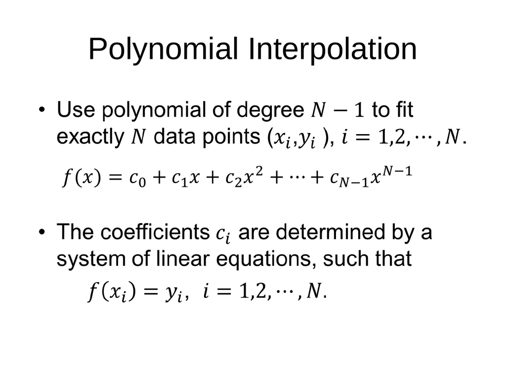
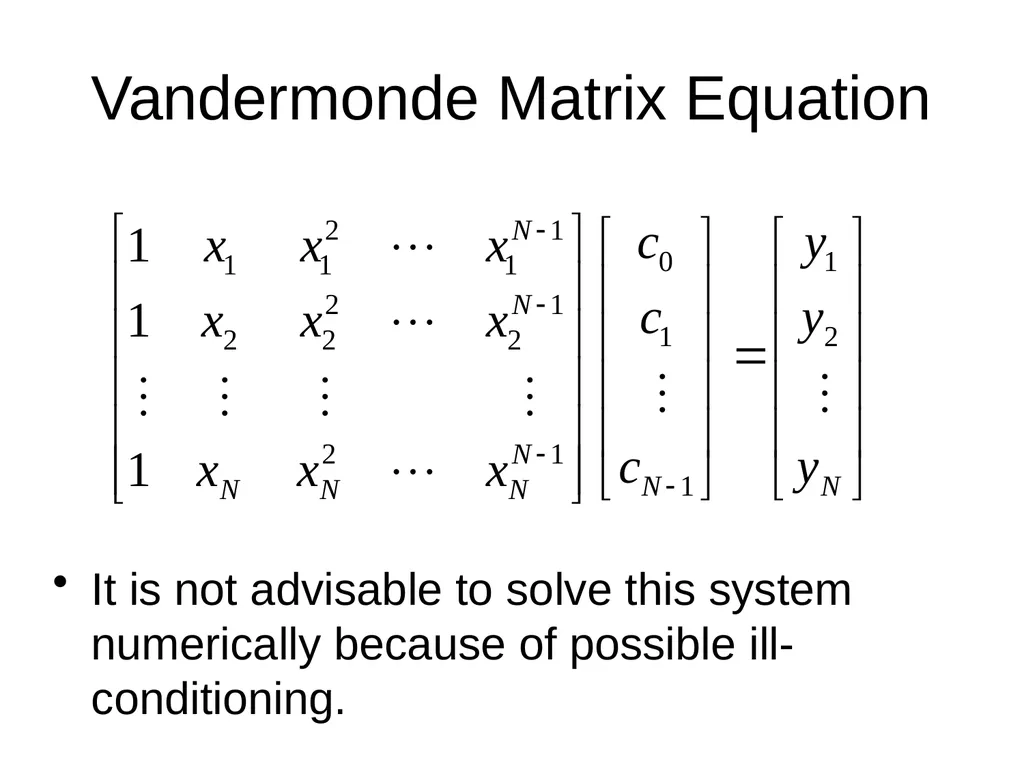
slide4. Vandermonde Matrix Equation It is not advisable to solve this system numerically because of possible ill-conditioning.<br>
slide5. Condition Number<br>
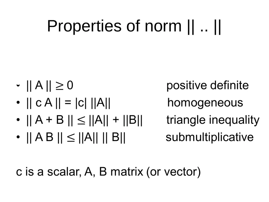
slide6. Properties of norm || .. ||<br>
slide7. Prove:<br>
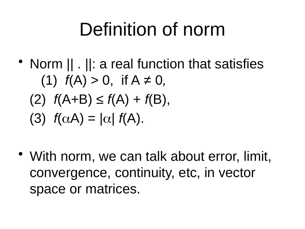
slide8. Definition of norm Norm || . ||: a real function that satisfies (1) f(A) > 0, if A ≠ 0,
(2) f(A+B) ≤ f(A) + f(B),
(3) f(A) = || f(A).

With norm, we can talk about error, limit, convergence, continuity, etc, in vector space or matrices.<br>
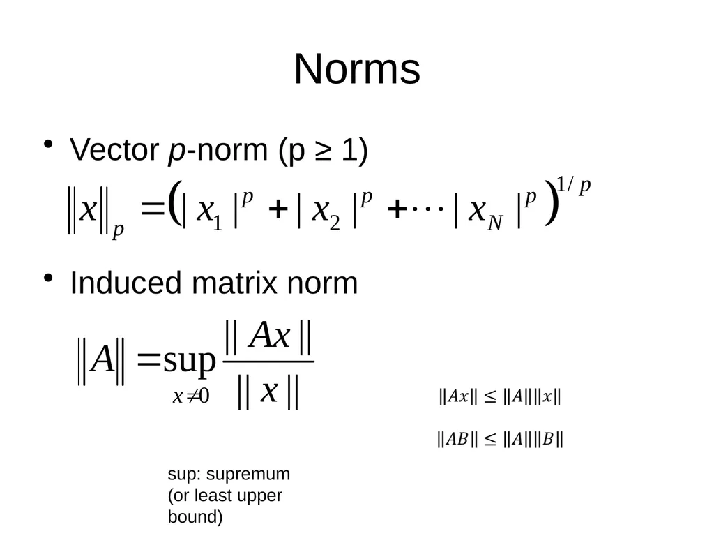
slide9. Norms Vector p-norm (p ≥ 1)

Induced matrix norm sup: supremum (or least upper bound)<br>
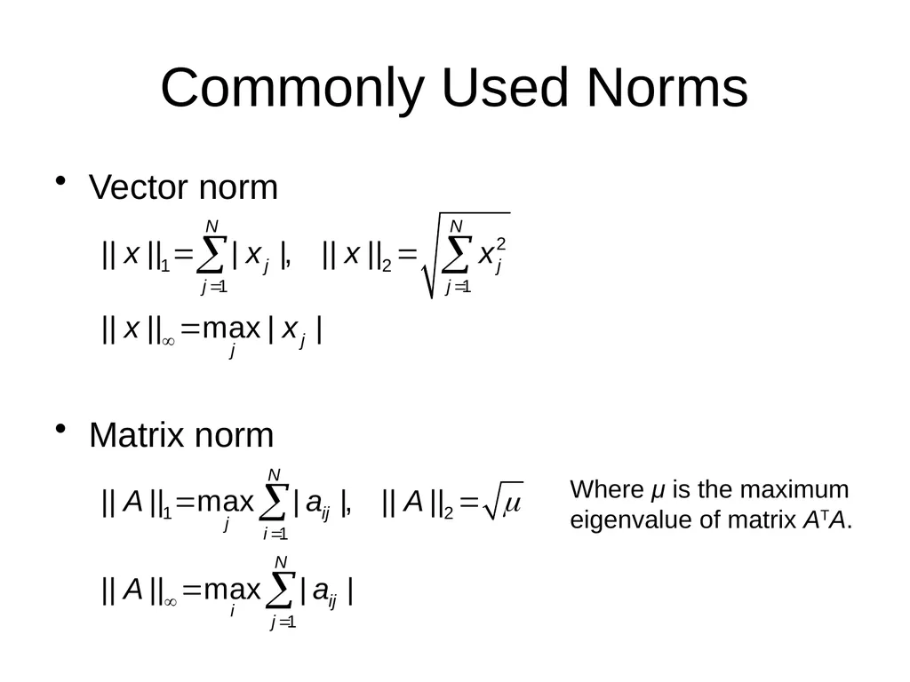
slide10. Commonly Used Norms Vector norm

Matrix norm Where μ is the maximum eigenvalue of matrix ATA.<br>
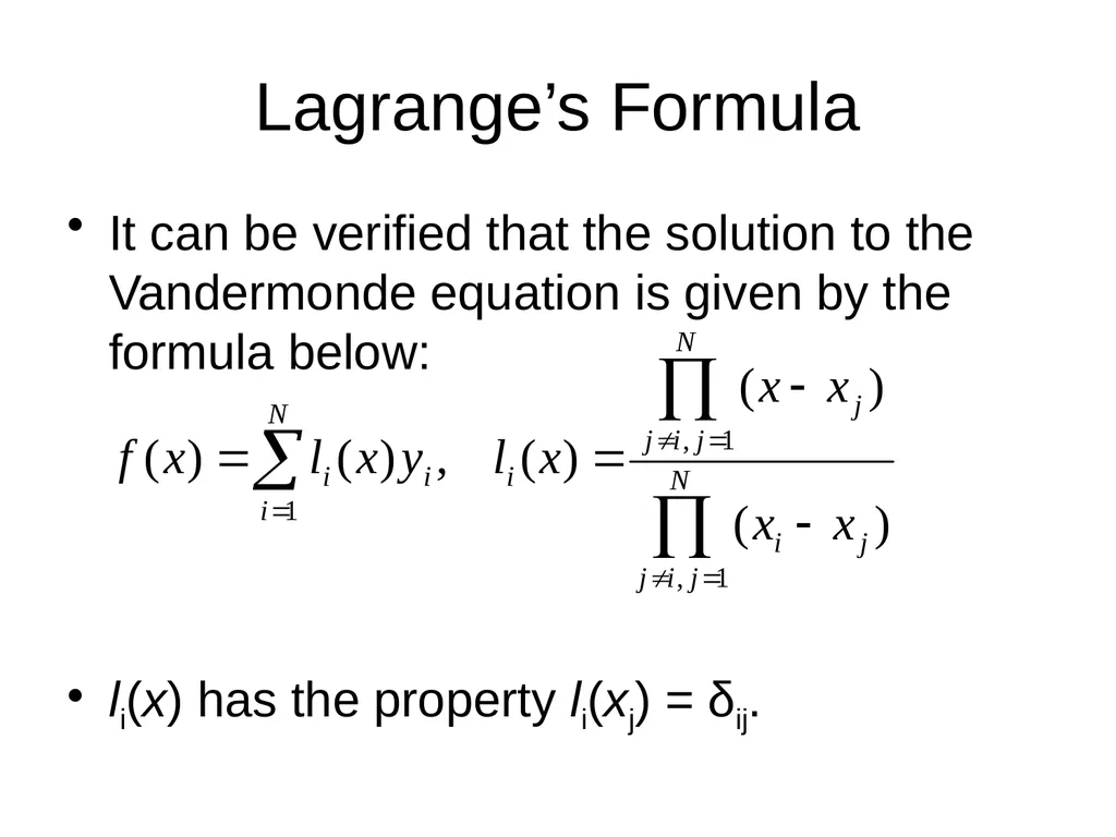
slide11. Lagrange’s Formula It can be verified that the solution to the Vandermonde equation is given by the formula below:

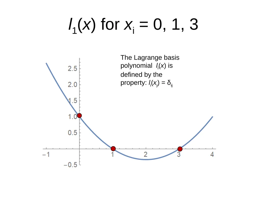
li(x) has the property li(xj) = δij.<br>
slide12. l1(x) for xi = 0, 1, 3 The Lagrange basis polynomial li(x) is defined by the property: li(xj) = δij<br>
slide13. Joseph-Louis Lagrange (1736-1813) Italian-French mathematician associated with many classic mathematics and physics – Lagrange multipliers in minimization of a function, Lagrange’s interpolation formula, Lagrange’s theorem in group theory and number theory, and the Lagrangian (L=T-V) in mechanics and Euler-Lagrange equations.<br>
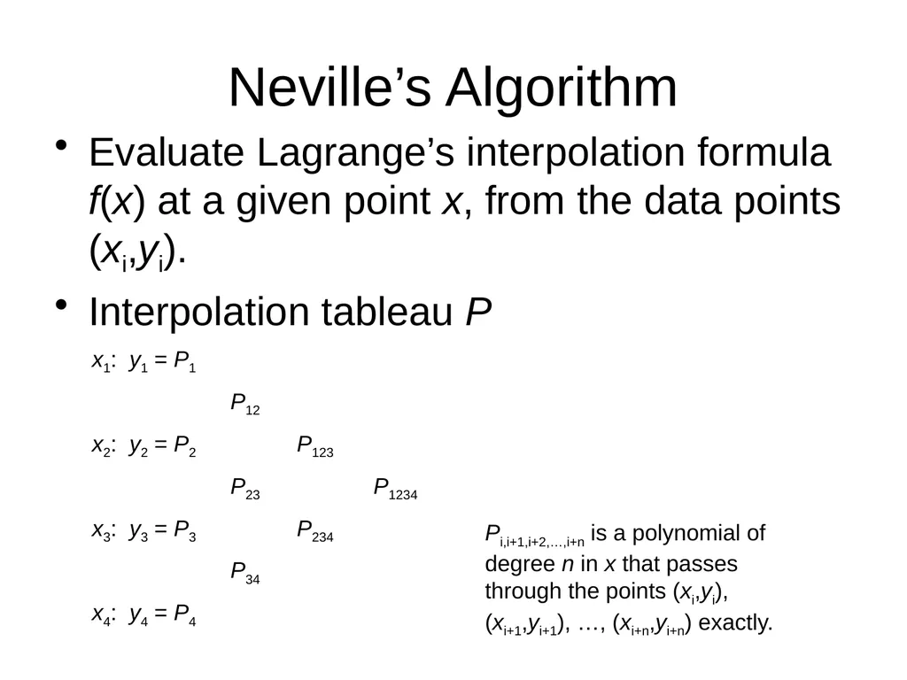
slide14. Neville’s Algorithm Evaluate Lagrange’s interpolation formula f(x) at a given point x, from the data points (xi,yi).
Interpolation tableau P x1: y1 = P1
P12
x2: y2 = P2 P123
P23 P1234
x3: y3 = P3 P234
P34
x4: y4 = P4 Pi,i+1,i+2,…,i+n is a polynomial of degree n in x that passes through the points (xi,yi), (xi+1,yi+1), …, (xi+n,yi+n) exactly.<br>
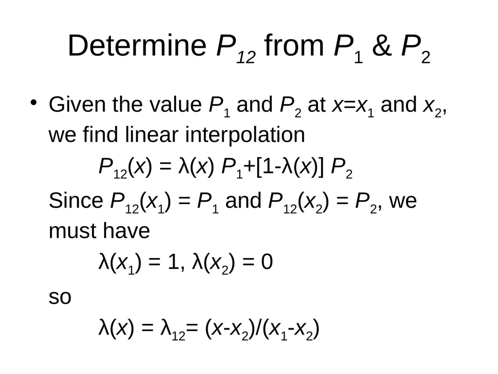
slide15. Determine P12 from P1 & P2 Given the value P1 and P2 at x=x1 and x2, we find linear interpolation
P12(x) = λ(x) P1+[1-λ(x)] P2
Since P12(x1) = P1 and P12(x2) = P2, we must have
λ(x1) = 1, λ(x2) = 0
so
λ(x) = λ12= (x-x2)/(x1-x2)<br>
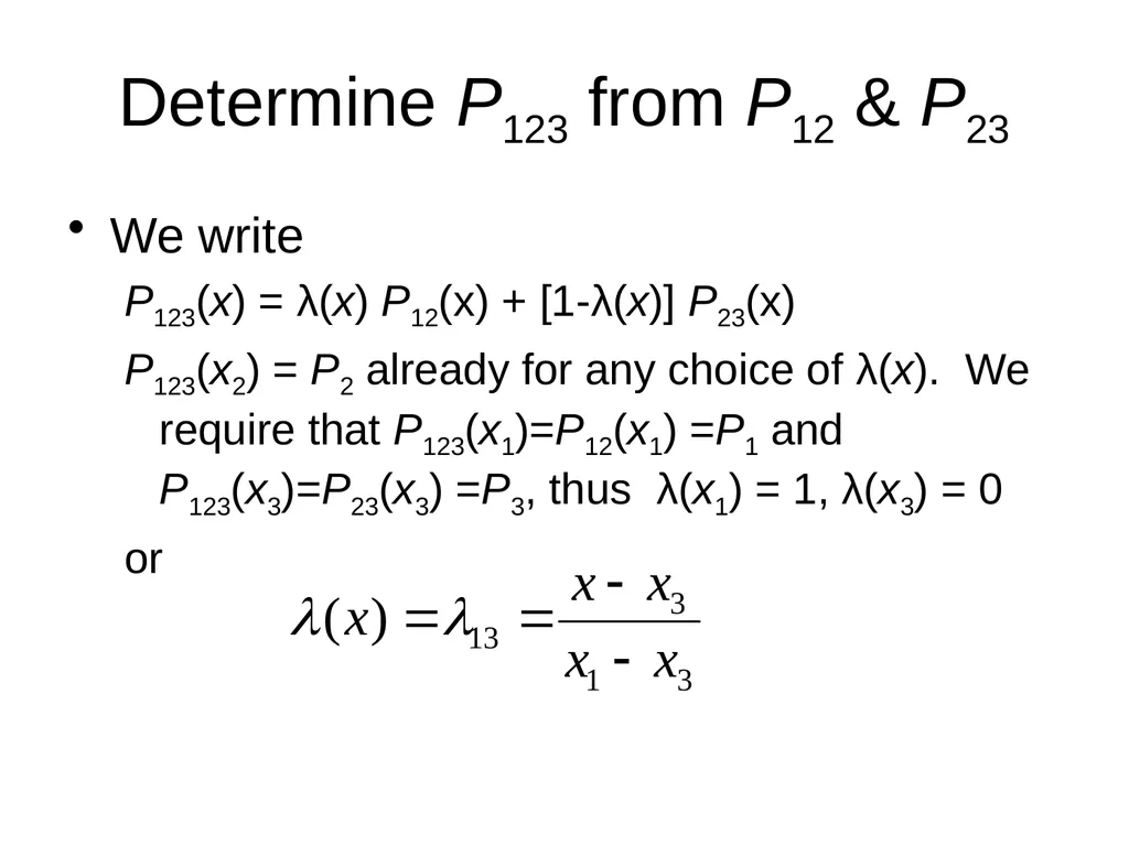
slide16. Determine P123 from P12 & P23 We write
P123(x) = λ(x) P12(x) + [1-λ(x)] P23(x)
P123(x2) = P2 already for any choice of λ(x). We require that P123(x1)=P12(x1) =P1 and P123(x3)=P23(x3) =P3, thus λ(x1) = 1, λ(x3) = 0
or<br>
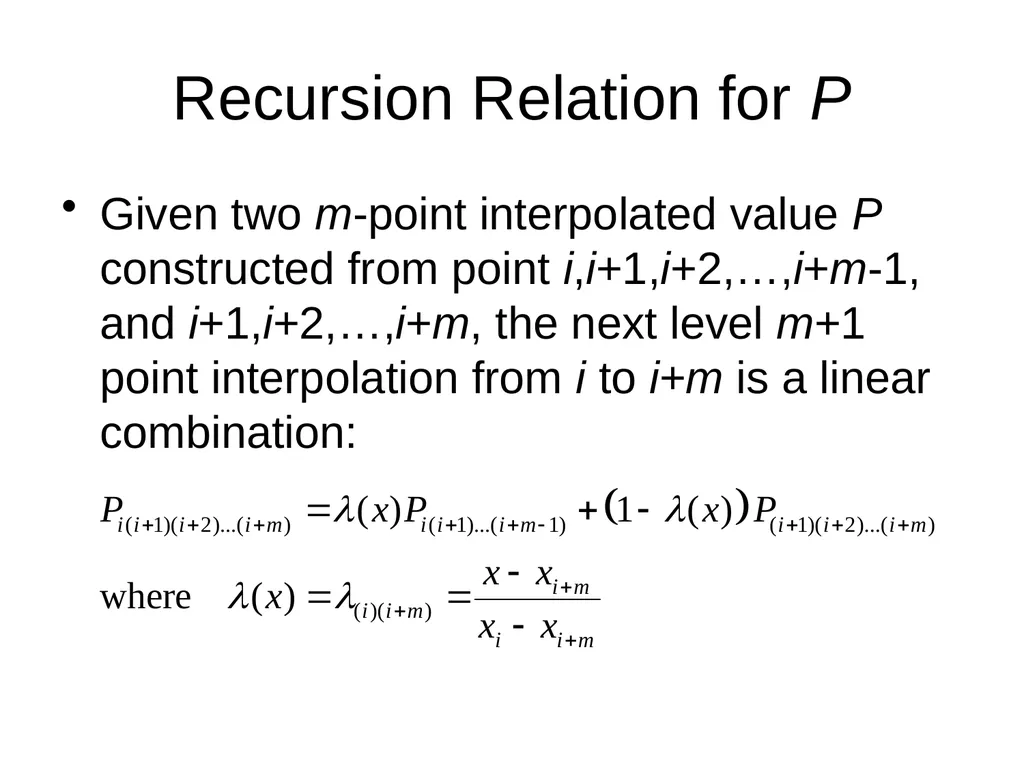
slide17. Recursion Relation for P Given two m-point interpolated value P constructed from point i,i+1,i+2,…,i+m-1, and i+1,i+2,…,i+m, the next level m+1 point interpolation from i to i+m is a linear combination:<br>
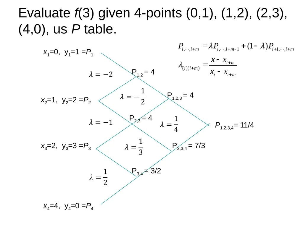
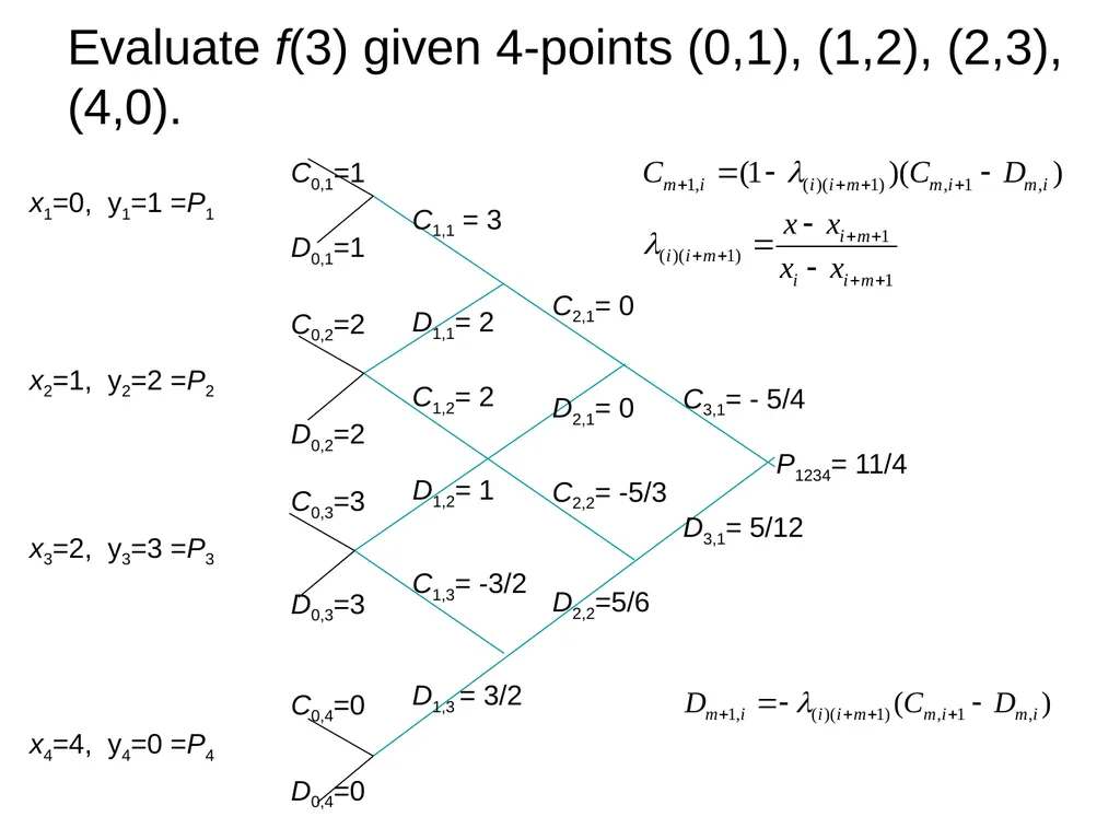
slide18. Evaluate f(3) given 4-points (0,1), (1,2), (2,3),(4,0), us P table. P1,2,3,4= 11/4 x1=0, y1=1 =P1 x2=1, y2=2 =P2 x3=2, y3=3 =P3 x4=4, y4=0 =P4 P1,2 = 4 P2,3 = 4 P3,4 = 3/2 P1,2,3 = 4 P2,3,4 = 7/3<br>
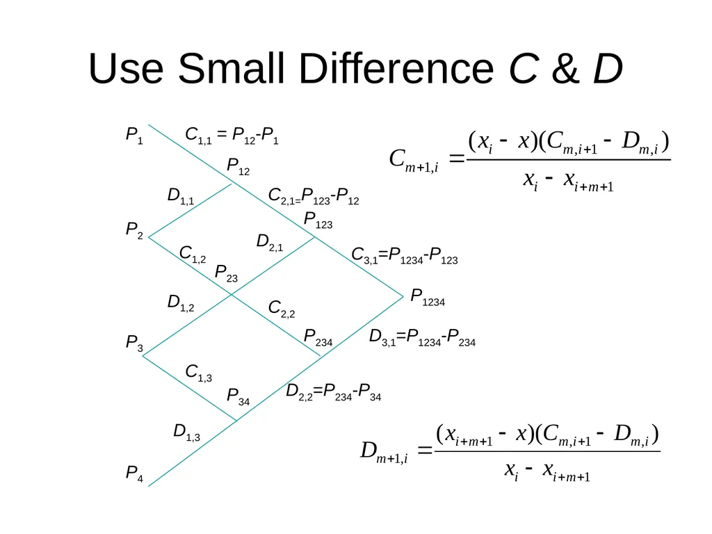
slide19. Use Small Difference C & D P1 P2 P3 P4 P12 P23 P34 P123 P234 P1234 C1,1 = P12-P1 D1,1 C1,2 C1,3 D1,2 D1,3 C2,1=P123-P12 C2,2 D2,1 C3,1=P1234-P123 D3,1=P1234-P234 D2,2=P234-P34<br>
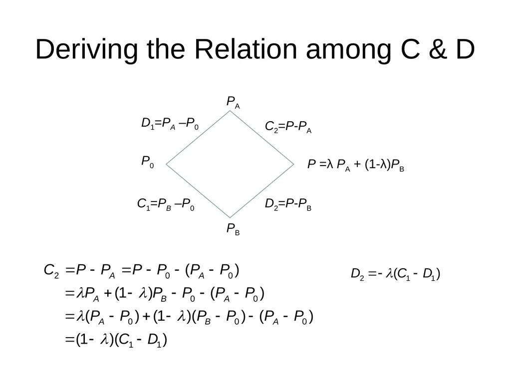
slide20. Deriving the Relation among C & D P =λ PA + (1-λ)PB PA PB P0 C2=P-PA C1=PB –P0 D2=P-PB D1=PA –P0<br>
slide21. Evaluate f(3) given 4-points (0,1), (1,2), (2,3),(4,0). P1234= 11/4 C1,1 = 3 D1,1= 2 C1,2= 2 C1,3= -3/2 D1,2= 1 D1,3 = 3/2 C2,1= 0 C2,2= -5/3 D2,1= 0 C3,1= - 5/4 D3,1= 5/12 D2,2=5/6 x1=0, y1=1 =P1 x2=1, y2=2 =P2 x3=2, y3=3 =P3 x4=4, y4=0 =P4 C0,1=1 D0,1=1 C0,2=2 D0,2=2 C0,3=3 D0,3=3 D0,4=0 C0,4=0<br>
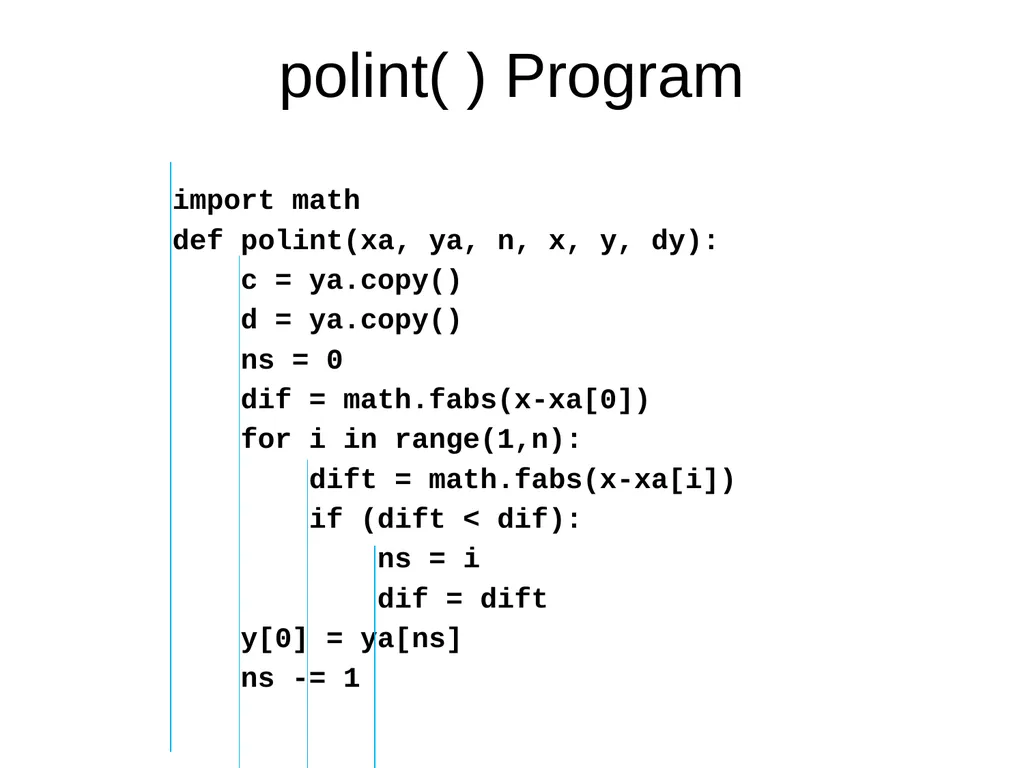
slide22. polint( ) Program import math
def polint(xa, ya, n, x, y, dy):
c = ya.copy()
d = ya.copy()
ns = 0
dif = math.fabs(x-xa[0])
for i in range(1,n):
dift = math.fabs(x-xa[i])
if (dift < dif):
ns = i
dif = dift
y[0] = ya[ns]
ns -= 1<br>
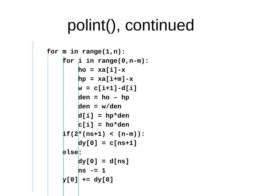
slide23. polint(), continued for m in range(1,n):
for i in range(0,n-m):
ho = xa[i]-x
hp = xa[i+m]-x
w = c[i+1]-d[i]
den = ho – hp
den = w/den
d[i] = hp*den
c[i] = ho*den
if(2*(ns+1) < (n-m)):
dy[0] = c[ns+1]
else:
dy[0] = d[ns]
ns -= 1
y[0] += dy[0]<br>
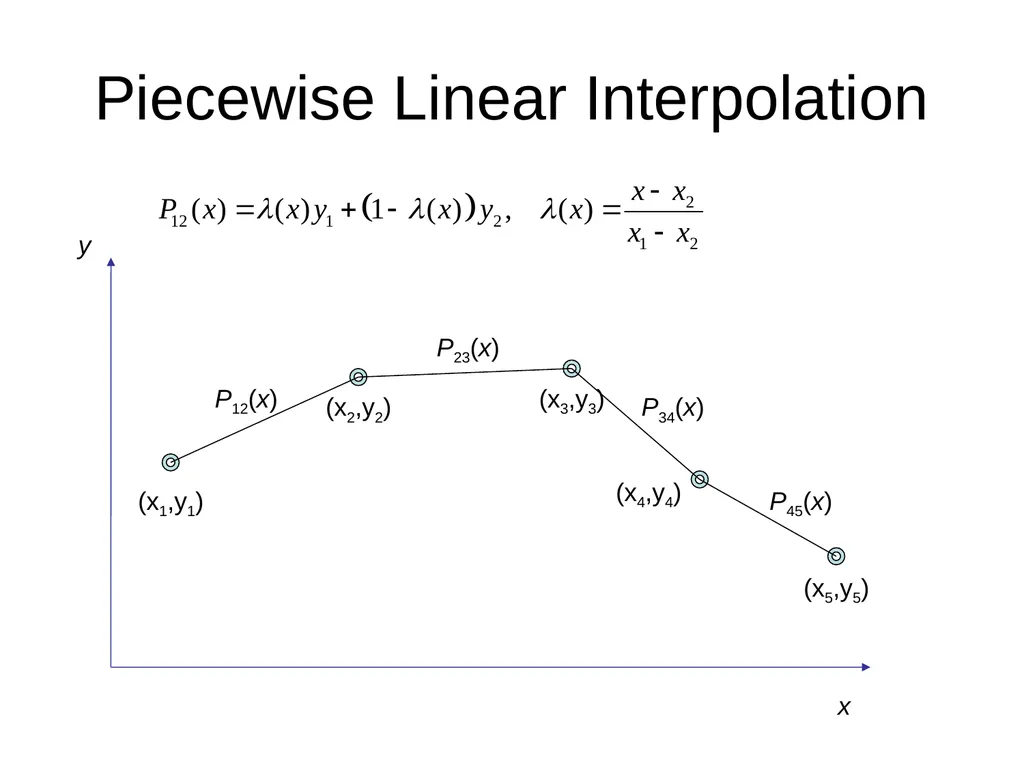
slide24. Piecewise Linear Interpolation (x1,y1) (x2,y2) (x3,y3) (x4,y4) (x5,y5) P12(x) P23(x) P34(x) P45(x) x y<br>
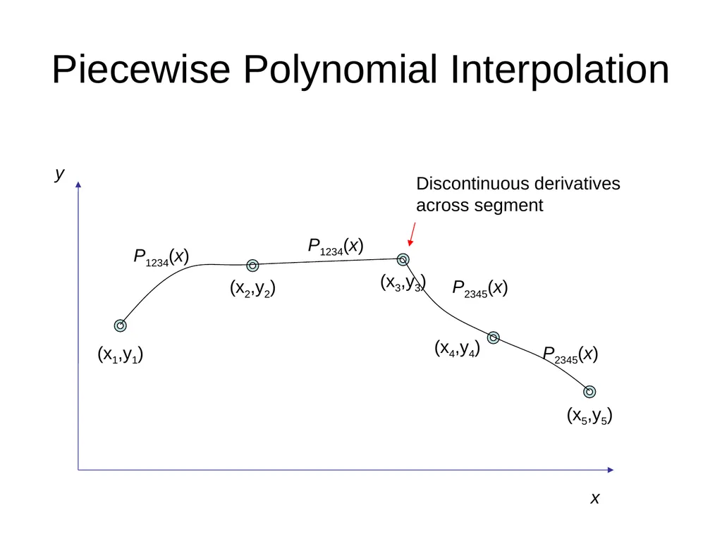
slide25. Piecewise Polynomial Interpolation (x1,y1) (x2,y2) (x3,y3) (x4,y4) (x5,y5) P1234(x) P1234(x) P2345(x) P2345(x) x y Discontinuous derivatives across segment<br>
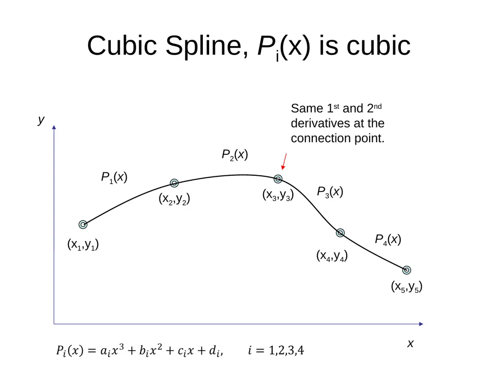
slide26. Cubic Spline, Pi(x) is cubic (x1,y1) (x2,y2) (x3,y3) (x4,y4) (x5,y5) P1(x) P2(x) P3(x) P4(x) x y Same 1st and 2nd derivatives at the connection point.<br>
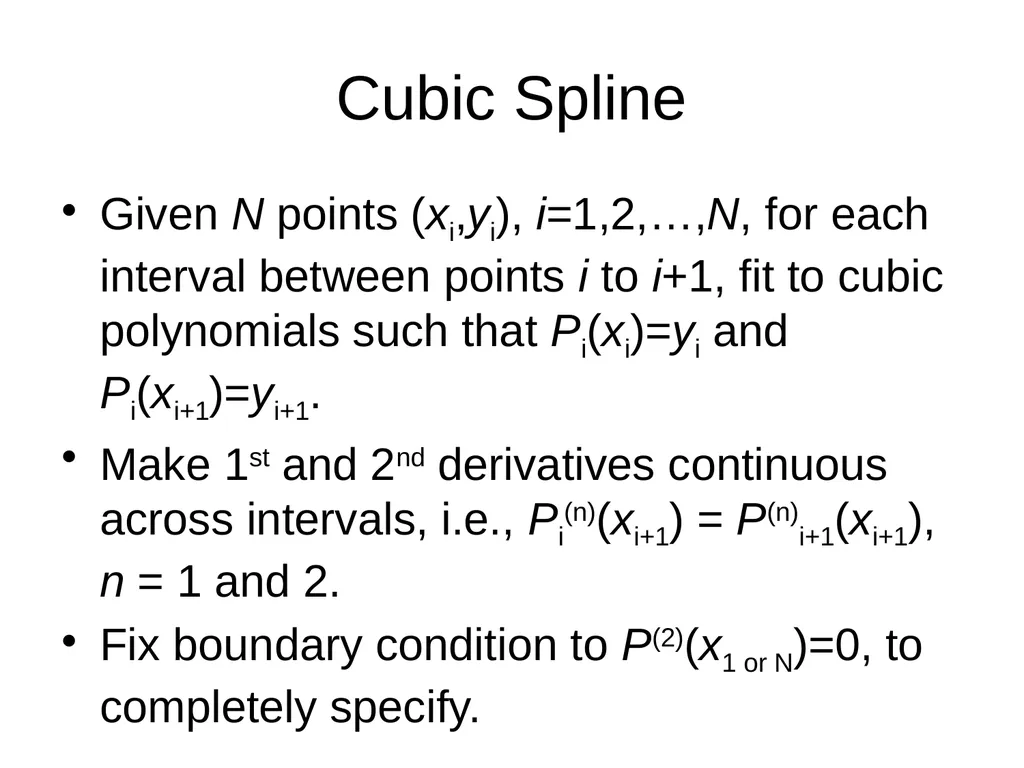
slide27. Cubic Spline Given N points (xi,yi), i=1,2,…,N, for each interval between points i to i+1, fit to cubic polynomials such that Pi(xi)=yi and Pi(xi+1)=yi+1.
Make 1st and 2nd derivatives continuous across intervals, i.e., Pi(n)(xi+1) = P(n)i+1(xi+1), n = 1 and 2.
Fix boundary condition to P(2)(x1 or N)=0, to completely specify.<br>
slide28. Reading NR, Chapter 3

See also J. Stoer and R. Bulirsch, “Introduction to Numerical Analysis,” Chapter 2.<br>