
Chapter 4 Search Fig. 4.1a Magic squares … Fig.


Description: Chapter 4 Search Fig. 4.1a Magic squares Fig. 4.1b and the eight queens problem Fig. 4.2 Towers of Hanoi Fig. 4.3 Generate and test finding solutions to the magic square p.40 inline image magic square partial solution Fig. 4.4 Magic
Related Topics
Download Presentation
"Chapter 4 Search Fig. 4.1a Magic squares … Fig." is the property of its rightful owner. Permission is granted to download and print the materials on this website for personal, non-commercial use only, and to display it on your personal computer provided you do not modify the materials and that you retain all copyright notices contained in the materials. By downloading content from our website, you accept the terms of this agreement.
Presentation Transcript
slide1. Chapter 4 Search<br>
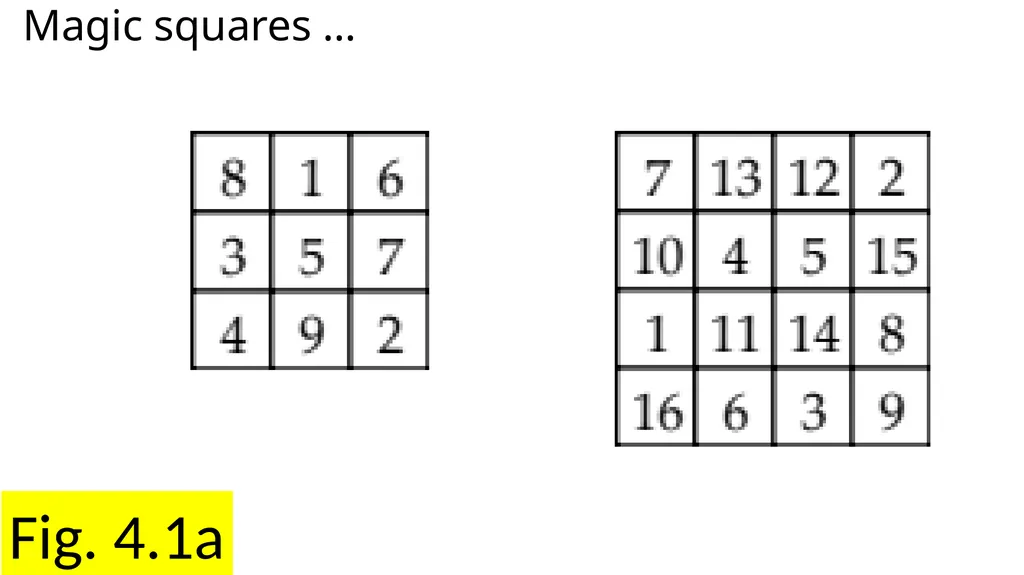
slide2. Fig. 4.1a Magic squares …<br>
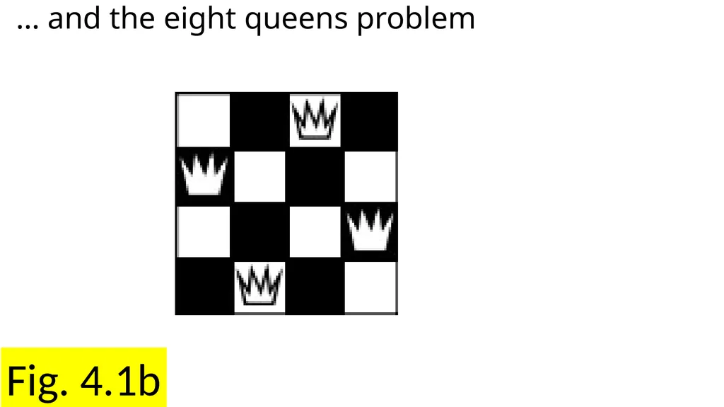
slide3. Fig. 4.1b … and the eight queens problem<br>
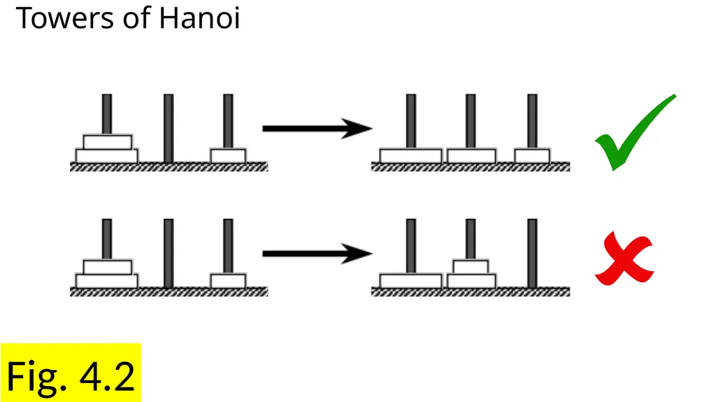
slide4. Fig. 4.2 Towers of Hanoi<br>
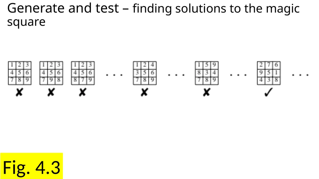
slide5. Fig. 4.3 Generate and test – finding solutions to the magic square<br>
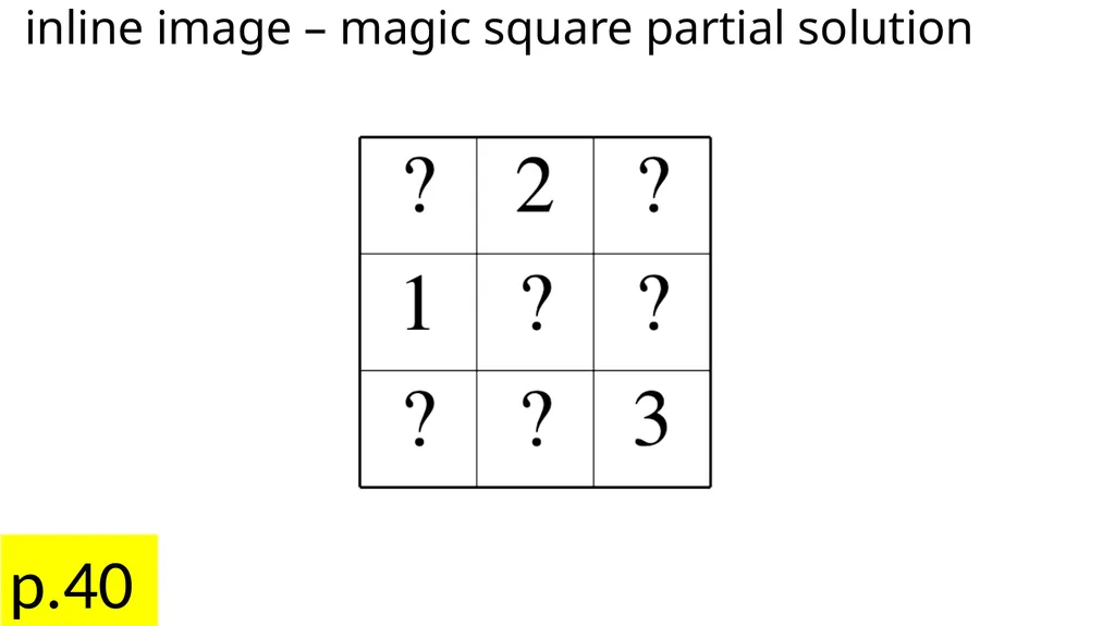
slide6. p.40 inline image – magic square partial solution<br>
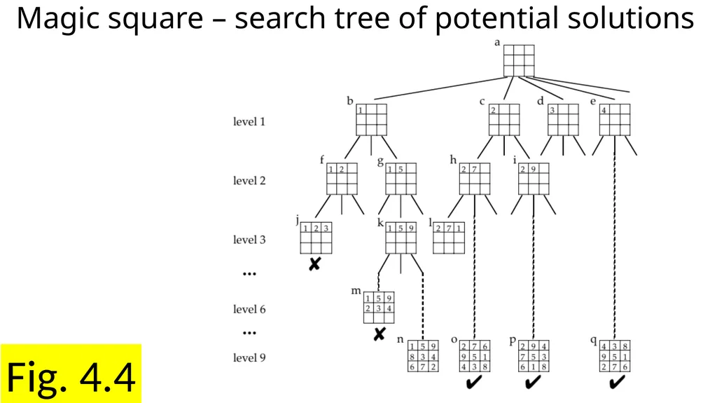
slide7. Fig. 4.4 Magic square – search tree of potential solutions<br>
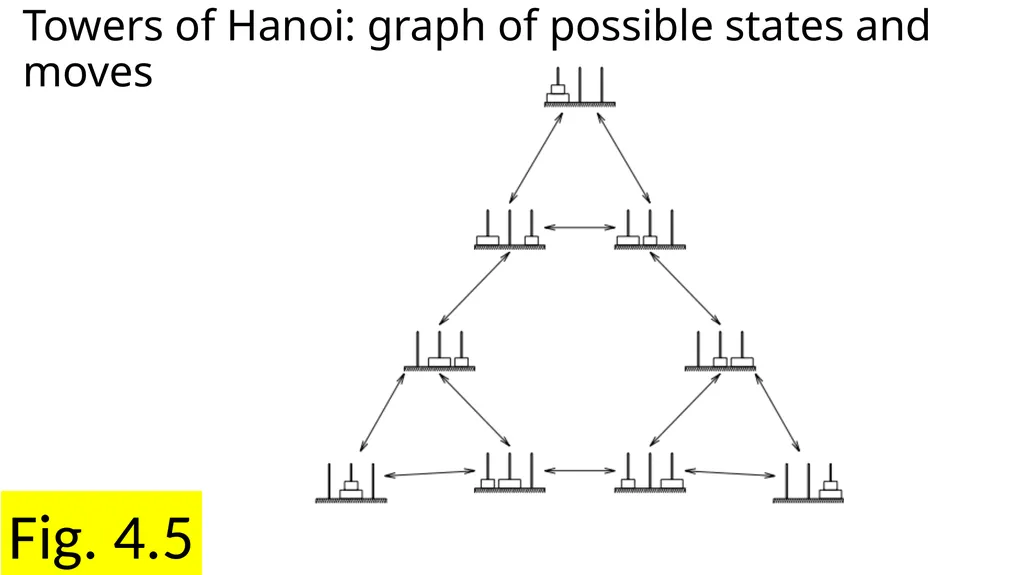
slide8. Fig. 4.5 Towers of Hanoi: graph of possible states and moves<br>
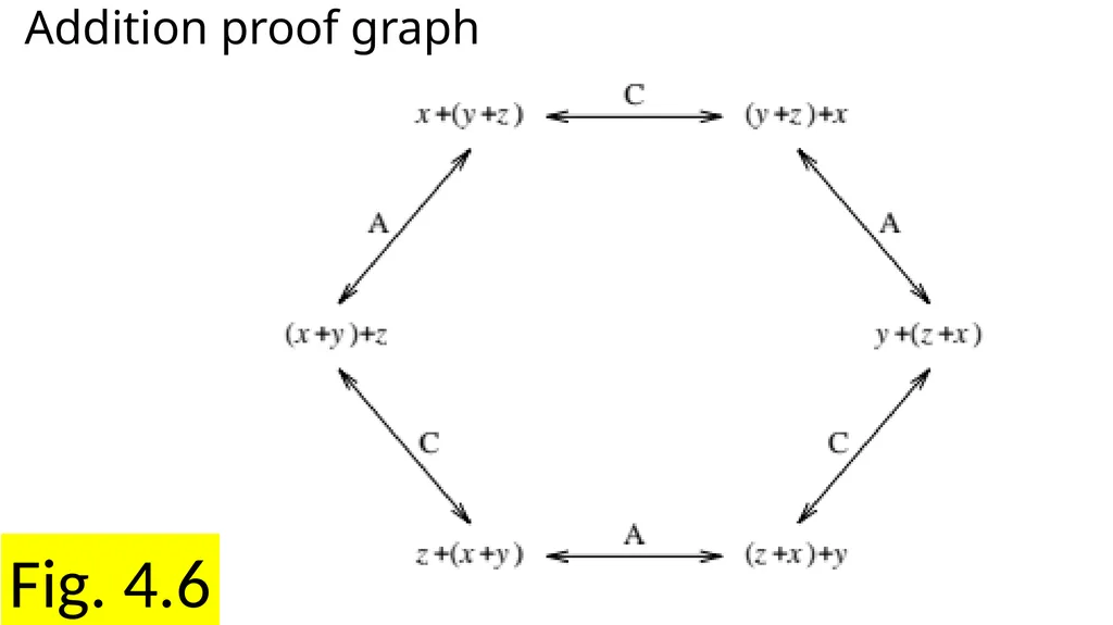
slide9. Fig. 4.6 Addition proof graph<br>
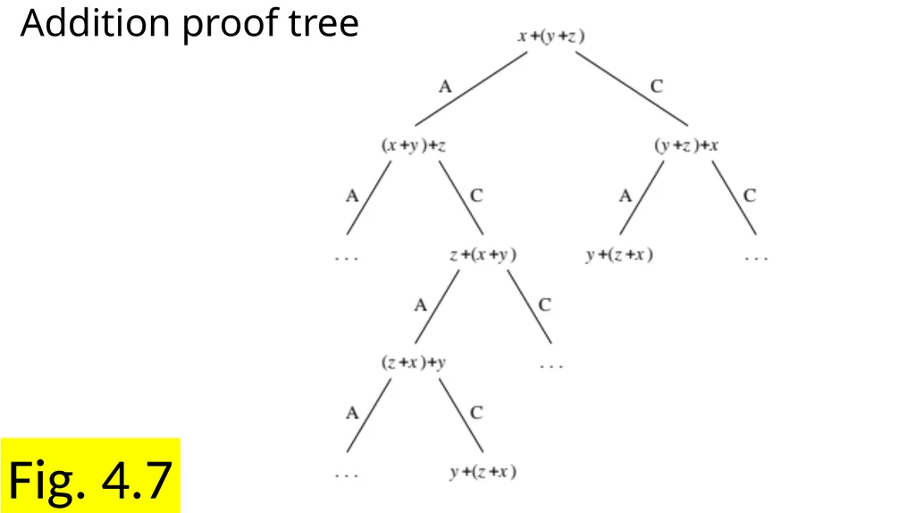
slide10. Fig. 4.7 Addition proof tree<br>
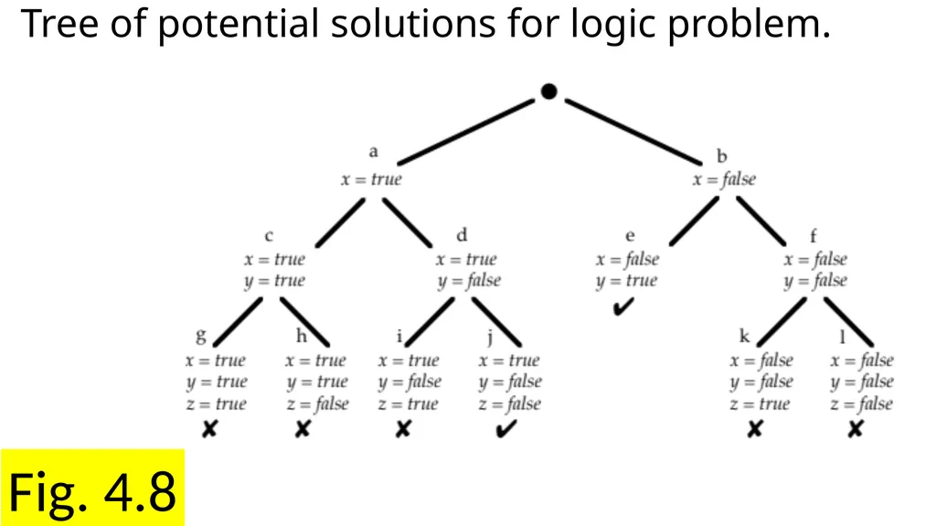
slide11. Fig. 4.8 Tree of potential solutions for logic problem.<br>
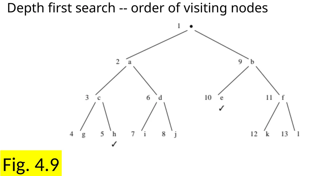
slide12. Fig. 4.9 Depth first search -- order of visiting nodes<br>
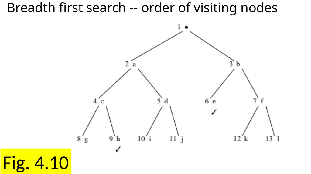
slide13. Fig. 4.10 Breadth first search -- order of visiting nodes<br>
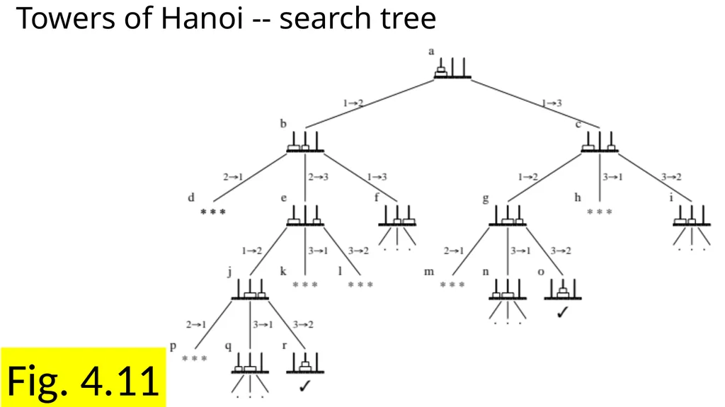
slide14. Fig. 4.11 Towers of Hanoi -- search tree<br>
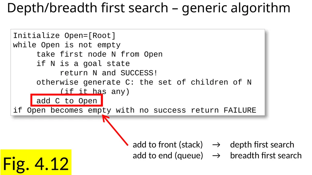
slide15. Fig. 4.12 Depth/breadth first search – generic algorithm Initialize Open=[Root]
while Open is not empty
take first node N from Open
if N is a goal state
return N and SUCCESS!
otherwise generate C: the set of children of N
(if it has any)
add C to Open
if Open becomes empty with no success return FAILURE add to front (stack) → depth first search
add to end (queue) → breadth first search<br>
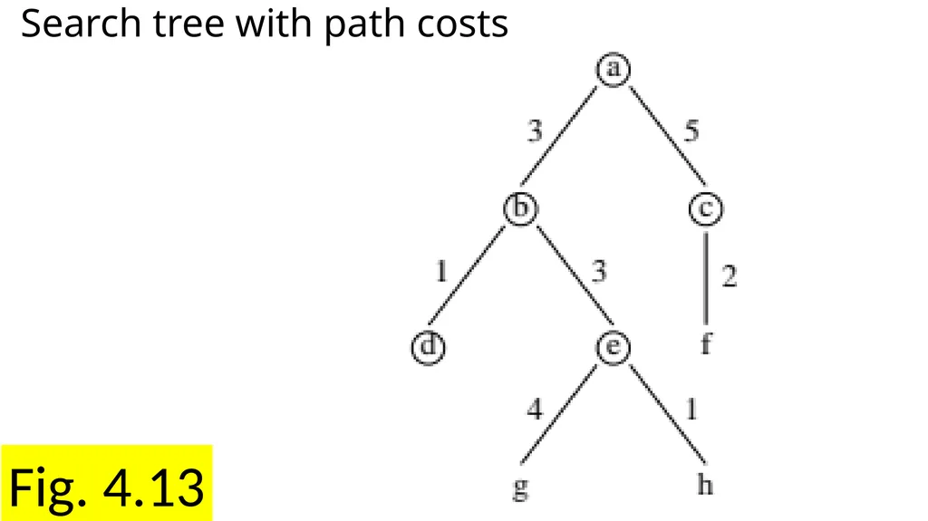
slide16. Fig. 4.13 Search tree with path costs<br>
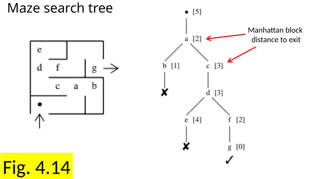
slide17. Fig. 4.14 Maze search tree Manhattan block distance to exit<br>
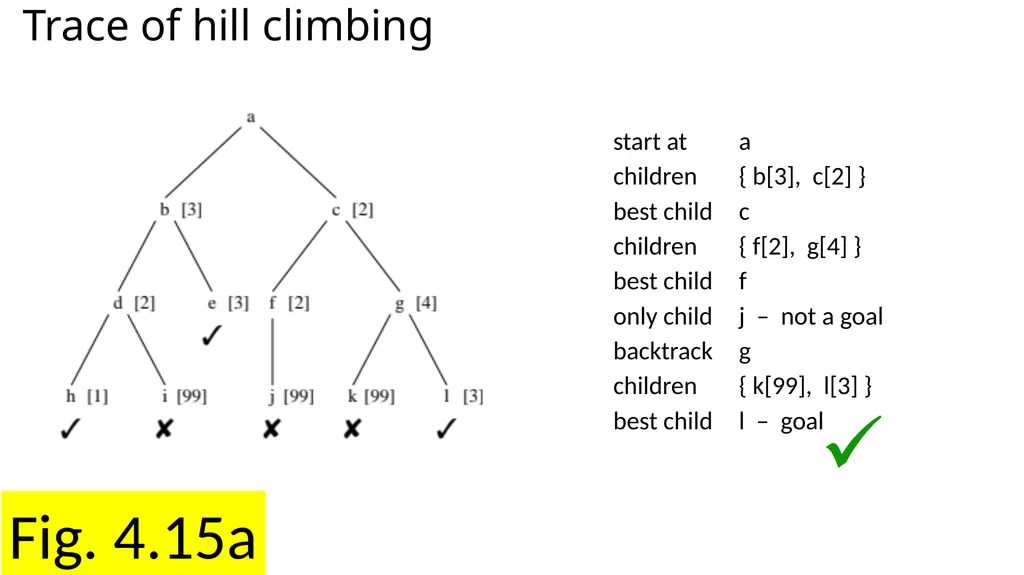
slide18. Fig. 4.15a Trace of hill climbing start at a
children { b[3], c[2] }
best child c
children { f[2], g[4] }
best child f
only child j – not a goal
backtrack g
children { k[99], l[3] }
best child l – goal<br>
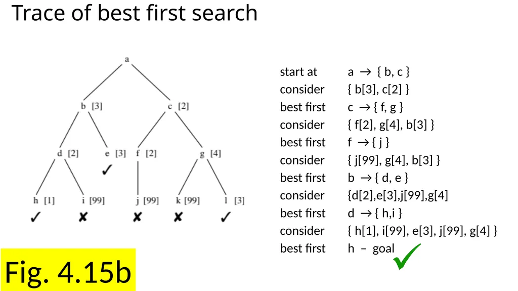
slide19. Fig. 4.15b Trace of best first search start at a → { b, c }
consider { b[3], c[2] }
best first c → { f, g }
consider { f[2], g[4], b[3] }
best first f → { j }
consider { j[99], g[4], b[3] }
best first b → { d, e }
consider {d[2],e[3],j[99],g[4]
best first d → { h,i }
consider { h[1], i[99], e[3], j[99], g[4] }
best first h – goal<br>
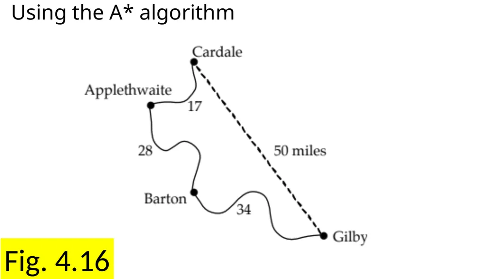
slide20. Fig. 4.16 Using the A* algorithm<br>
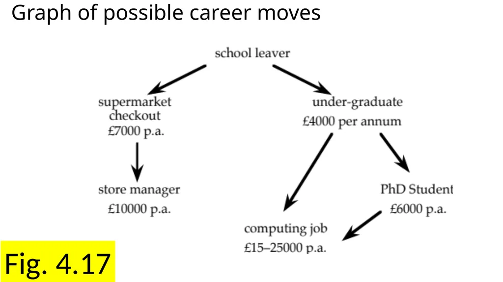
slide21. Fig. 4.17 Graph of possible career moves<br>
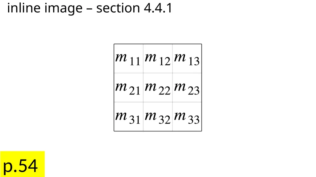
slide22. p.54 inline image – section 4.4.1<br>
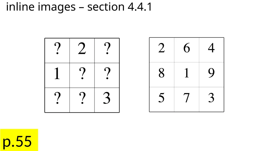
slide23. p.55 inline images – section 4.4.1<br>
slide2. Fig. 4.1a Magic squares …<br>
slide3. Fig. 4.1b … and the eight queens problem<br>
slide4. Fig. 4.2 Towers of Hanoi<br>
slide5. Fig. 4.3 Generate and test – finding solutions to the magic square<br>
slide6. p.40 inline image – magic square partial solution<br>
slide7. Fig. 4.4 Magic square – search tree of potential solutions<br>
slide8. Fig. 4.5 Towers of Hanoi: graph of possible states and moves<br>
slide9. Fig. 4.6 Addition proof graph<br>
slide10. Fig. 4.7 Addition proof tree<br>
slide11. Fig. 4.8 Tree of potential solutions for logic problem.<br>
slide12. Fig. 4.9 Depth first search -- order of visiting nodes<br>
slide13. Fig. 4.10 Breadth first search -- order of visiting nodes<br>
slide14. Fig. 4.11 Towers of Hanoi -- search tree<br>
slide15. Fig. 4.12 Depth/breadth first search – generic algorithm Initialize Open=[Root]
while Open is not empty
take first node N from Open
if N is a goal state
return N and SUCCESS!
otherwise generate C: the set of children of N
(if it has any)
add C to Open
if Open becomes empty with no success return FAILURE add to front (stack) → depth first search
add to end (queue) → breadth first search<br>
slide16. Fig. 4.13 Search tree with path costs<br>
slide17. Fig. 4.14 Maze search tree Manhattan block distance to exit<br>
slide18. Fig. 4.15a Trace of hill climbing start at a
children { b[3], c[2] }
best child c
children { f[2], g[4] }
best child f
only child j – not a goal
backtrack g
children { k[99], l[3] }
best child l – goal<br>
slide19. Fig. 4.15b Trace of best first search start at a → { b, c }
consider { b[3], c[2] }
best first c → { f, g }
consider { f[2], g[4], b[3] }
best first f → { j }
consider { j[99], g[4], b[3] }
best first b → { d, e }
consider {d[2],e[3],j[99],g[4]
best first d → { h,i }
consider { h[1], i[99], e[3], j[99], g[4] }
best first h – goal<br>
slide20. Fig. 4.16 Using the A* algorithm<br>
slide21. Fig. 4.17 Graph of possible career moves<br>
slide22. p.54 inline image – section 4.4.1<br>
slide23. p.55 inline images – section 4.4.1<br>