
Chapter 7 Demand Forecasting in a Supply Chain
Description: Chapter 7 Demand Forecasting in a Supply Chain Forecasting -1 Moving Average Ardavan Asef-Vaziri Based on Operations management: Stevenson Operations Management: Jacobs, Chase, and Aquilano Supply Chain Management: Chopra and Meindl USC
Related Topics
Download Presentation
"Chapter 7 Demand Forecasting in a Supply Chain" is the property of its rightful owner. Permission is granted to download and print the materials on this website for personal, non-commercial use only, and to display it on your personal computer provided you do not modify the materials and that you retain all copyright notices contained in the materials. By downloading content from our website, you accept the terms of this agreement.
Presentation Transcript
slide1. Chapter 7
Demand Forecasting
in a Supply Chain Forecasting -1
Moving Average
Ardavan Asef-Vaziri
Based on
Operations management: Stevenson
Operations Management: Jacobs, Chase, and Aquilano
Supply Chain Management: Chopra and Meindl
USC Marshall School of Business Lecture Notes
“Those who do not remember the past are condemned to repeat it”
George Santayana Spanish philosopher, essayist, poet and novelist (1863-1952)<br>
slide2. Recoded Lecture on Moving Average Slides https://www.youtube.com/watch?v=gt-YOLxJqBk&t=8s<br>
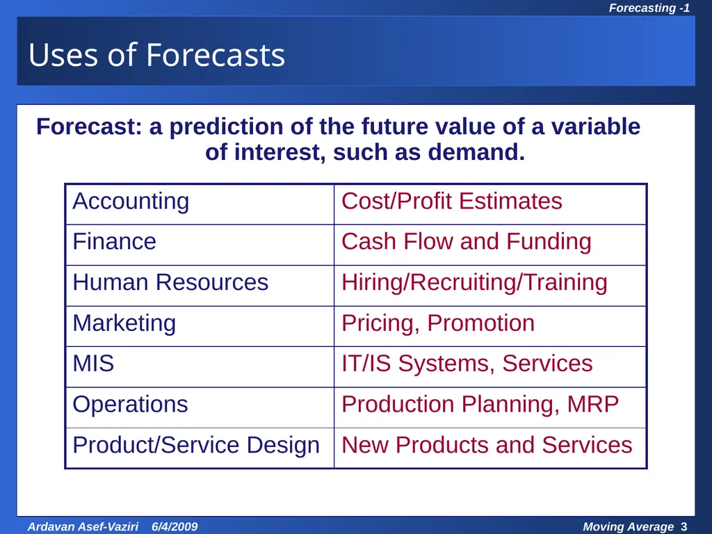
slide3. Uses of Forecasts Forecast: a prediction of the future value of a variable of interest, such as demand.<br>
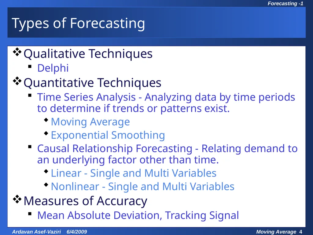
slide4. Types of Forecasting Qualitative Techniques
Delphi
Quantitative Techniques
Time Series Analysis - Analyzing data by time periods to determine if trends or patterns exist.
Moving Average
Exponential Smoothing
Causal Relationship Forecasting - Relating demand to an underlying factor other than time.
Linear - Single and Multi Variables
Nonlinear - Single and Multi Variables
Measures of Accuracy
Mean Absolute Deviation, Tracking Signal<br>
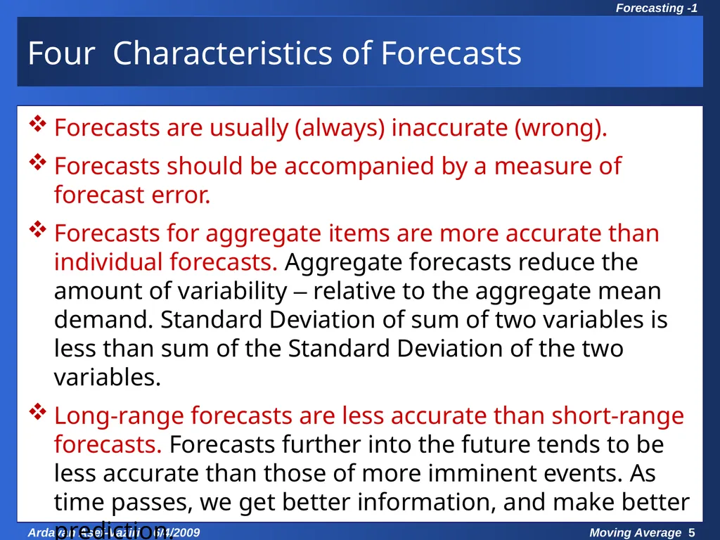
slide5. Four Characteristics of Forecasts Forecasts are usually (always) inaccurate (wrong).
Forecasts should be accompanied by a measure of forecast error.
Forecasts for aggregate items are more accurate than individual forecasts. Aggregate forecasts reduce the amount of variability – relative to the aggregate mean demand. Standard Deviation of sum of two variables is less than sum of the Standard Deviation of the two variables.
Long-range forecasts are less accurate than short-range forecasts. Forecasts further into the future tends to be less accurate than those of more imminent events. As time passes, we get better information, and make better prediction.<br>
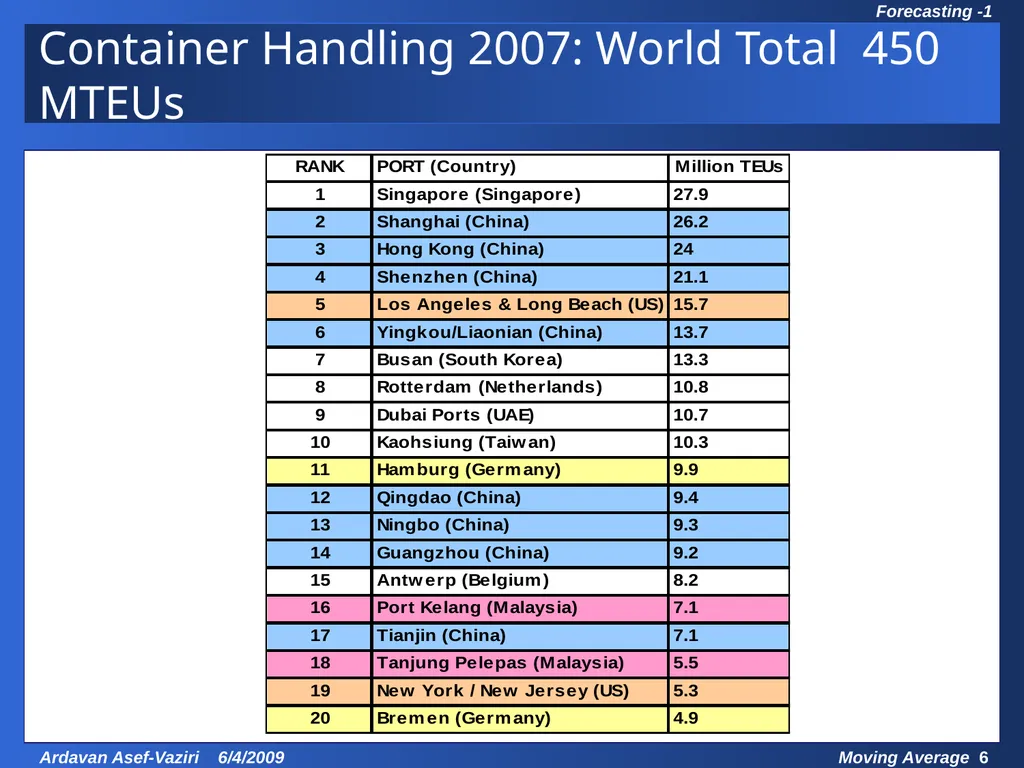
slide6. Container Handling 2007: World Total 450 MTEUs<br>
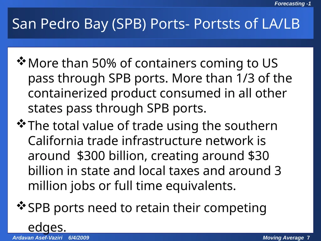
slide7. San Pedro Bay (SPB) Ports- Portsts of LA/LB More than 50% of containers coming to US pass through SPB ports. More than 1/3 of the containerized product consumed in all other states pass through SPB ports.
The total value of trade using the southern California trade infrastructure network is around $300 billion, creating around $30 billion in state and local taxes and around 3 million jobs or full time equivalents.
SPB ports need to retain their competing edges.<br>
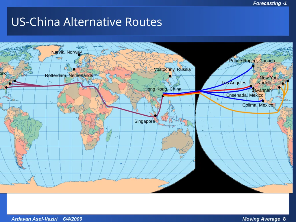
slide8. US-China Alternative Routes Narvik, Norway Vostochny, Russia Hong Kong, China Singapore Rotterdam, Netherlands Savannah Norfolk New York Prince Rupert, Canada Savannah Norfolk New York Los Angeles Colima, Mexico Ensenada, Mexico<br>
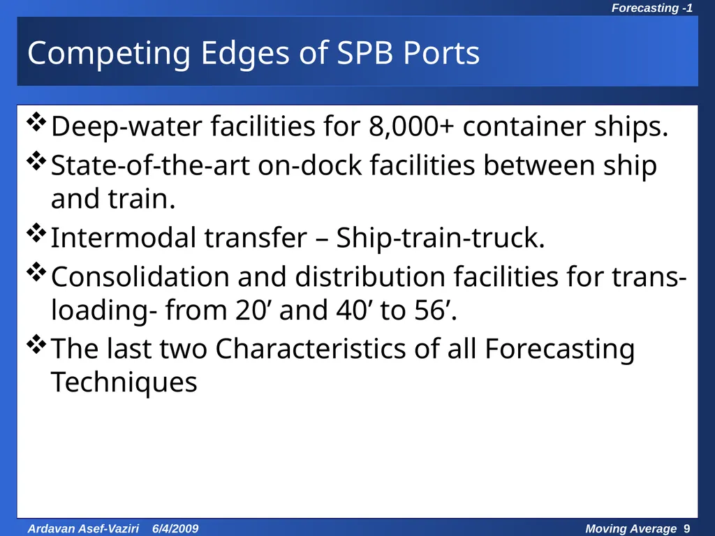
slide9. Competing Edges of SPB Ports Deep-water facilities for 8,000+ container ships.
State-of-the-art on-dock facilities between ship and train.
Intermodal transfer – Ship-train-truck.
Consolidation and distribution facilities for trans-loading- from 20’ and 40’ to 56’.
The last two Characteristics of all Forecasting Techniques<br>
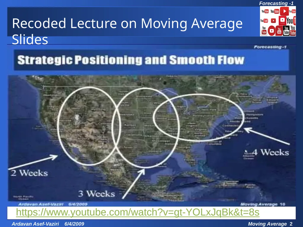
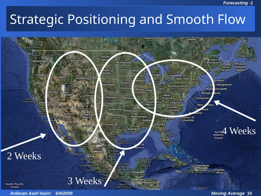
slide10. Strategic Positioning and Smooth Flow<br>
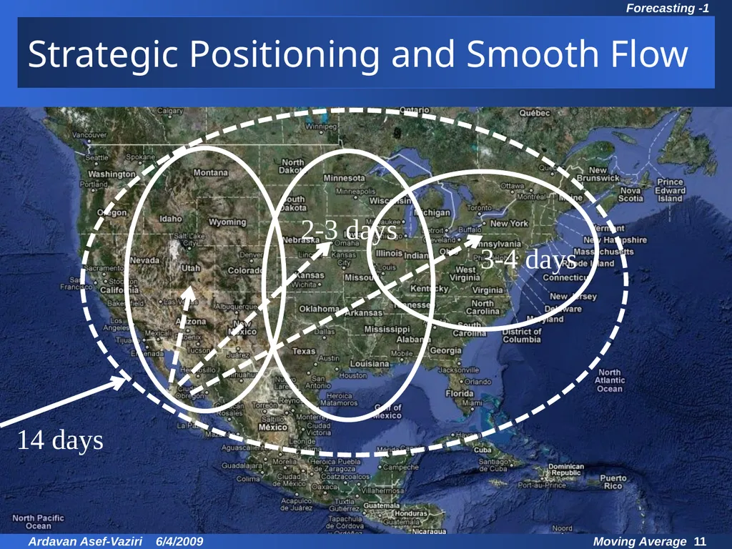
slide11. Strategic Positioning and Smooth Flow<br>
slide12. Qualitative Methods - Delphi Non-quantitative forecasting techniques based on expert opinions and intuition. Typically used when there are no data available.
Delphi Method
Subjective, judgmental
Based on intuition, estimates, and opinions
Expert Opinions
Market Research
Historical Analogies<br>
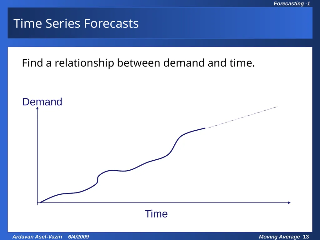
slide13. Find a relationship between demand and time. Demand Time Time Series Forecasts<br>
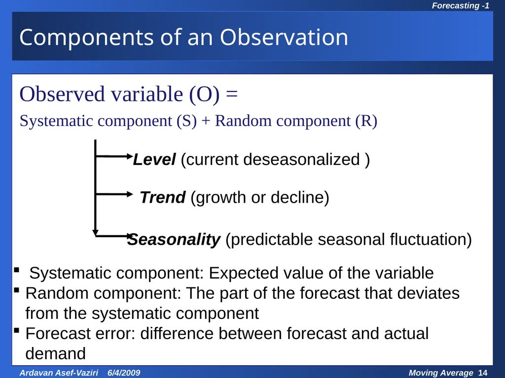
slide14. Components of an Observation Observed variable (O) =
Systematic component (S) + Random component (R) Level (current deseasonalized ) Trend (growth or decline) Seasonality (predictable seasonal fluctuation) Systematic component: Expected value of the variable
Random component: The part of the forecast that deviates from the systematic component
Forecast error: difference between forecast and actual demand<br>
slide15. Naive Forecast
Moving Average
Exponential Smoothing Time Series Techniques<br>
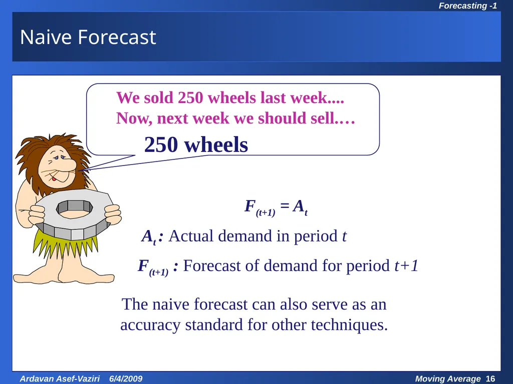
slide16. We sold 250 wheels last week....
Now, next week we should sell.… At : Actual demand in period t F(t+1) : Forecast of demand for period t+1 F(t+1) = At Naive Forecast 250 wheels The naive forecast can also serve as an
accuracy standard for other techniques.<br>
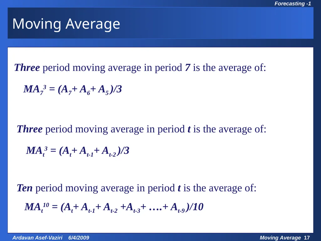
slide17. Moving Average Three period moving average in period 7 is the average of: MAt10 = (At+ At-1+ At-2 +At-3+ ….+ At-9 )/10 MA73 = (A7+ A6+ A5 )/3 Three period moving average in period t is the average of: MAt3 = (At+ At-1+ At-2 )/3 Ten period moving average in period t is the average of:<br>
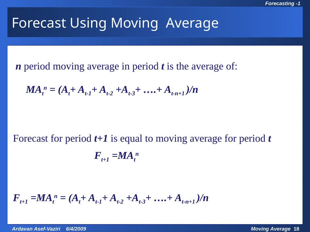
slide18. Forecast Using Moving Average Forecast for period t+1 is equal to moving average for period t Ft+1 =MAtn n period moving average in period t is the average of: MAtn = (At+ At-1+ At-2 +At-3+ ….+ At-n+1 )/n Ft+1 =MAtn = (At+ At-1+ At-2 +At-3+ ….+ At-n+1 )/n<br>
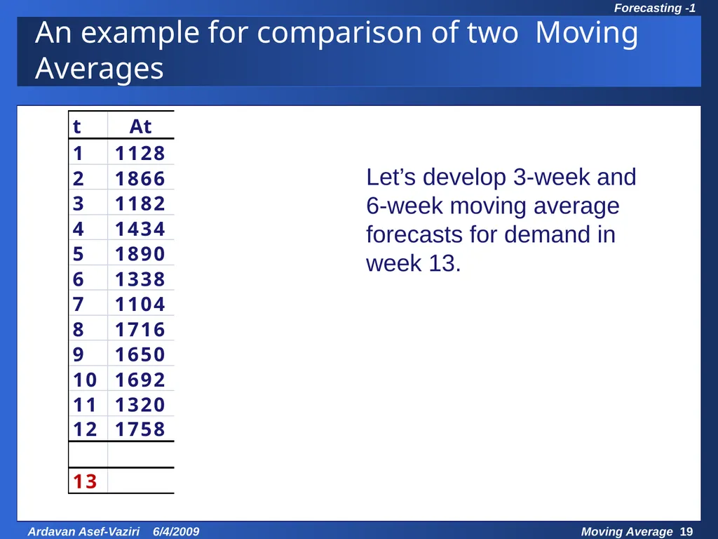
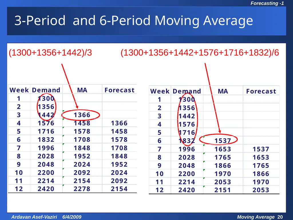
slide19. An example for comparison of two Moving Averages Let’s develop 3-week and 6-week moving average forecasts for demand in week 13.<br>
slide20. 3-Period and 6-Period Moving Average<br>
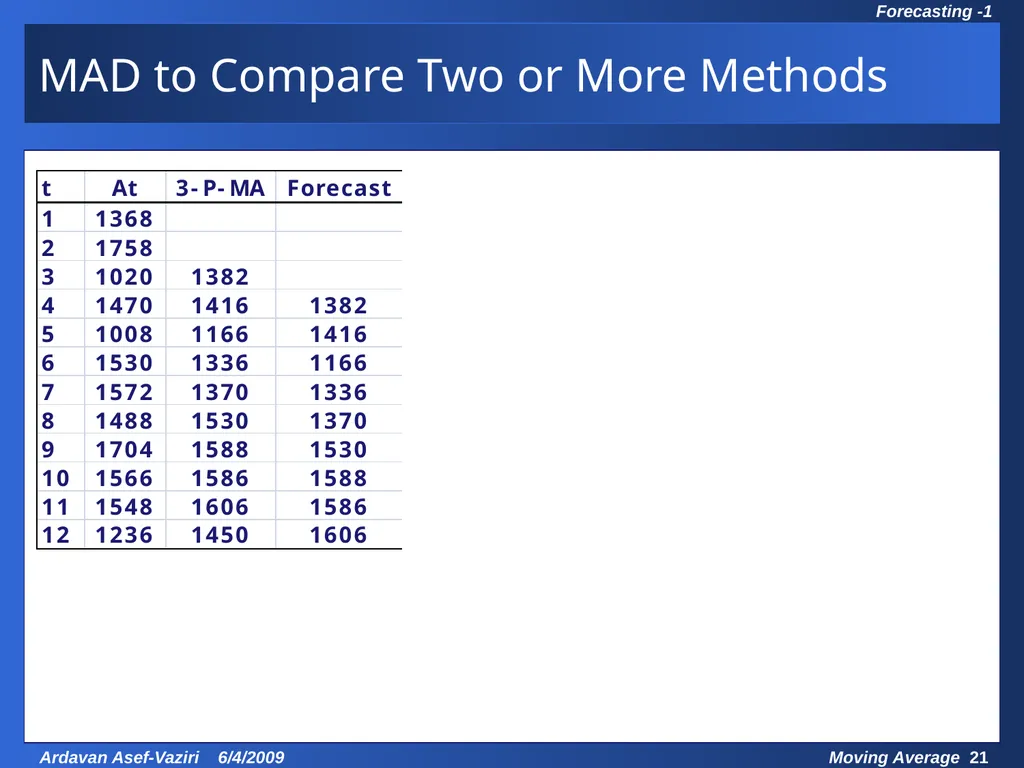
slide21. MAD to Compare Two or More Methods<br>
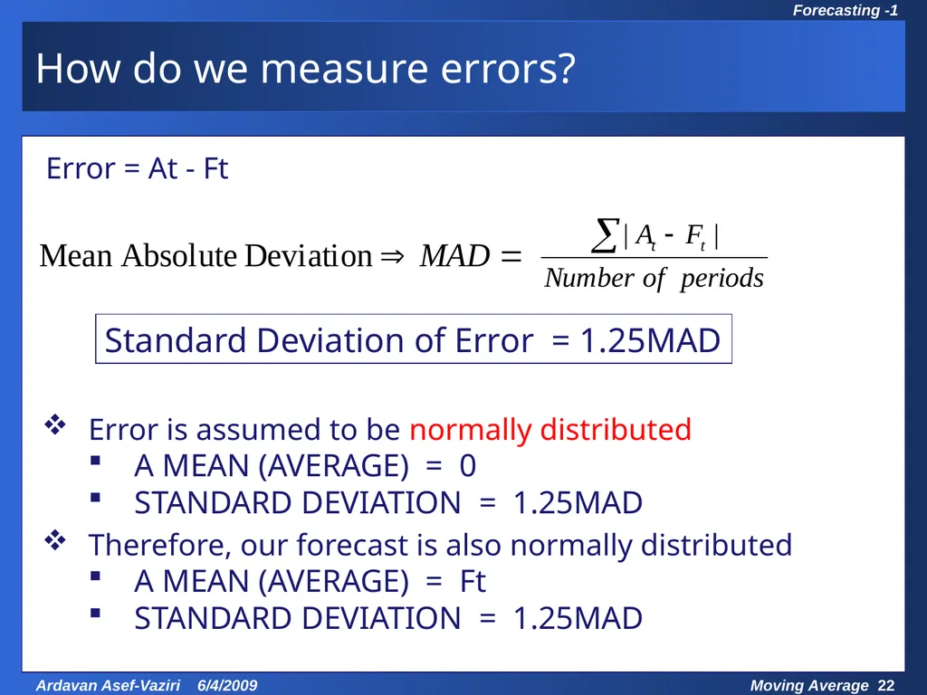
slide22. How do we measure errors? Standard Deviation of Error = 1.25MAD Error is assumed to be normally distributed
A MEAN (AVERAGE) = 0
STANDARD DEVIATION = 1.25MAD
Therefore, our forecast is also normally distributed
A MEAN (AVERAGE) = Ft
STANDARD DEVIATION = 1.25MAD Error = At - Ft<br>
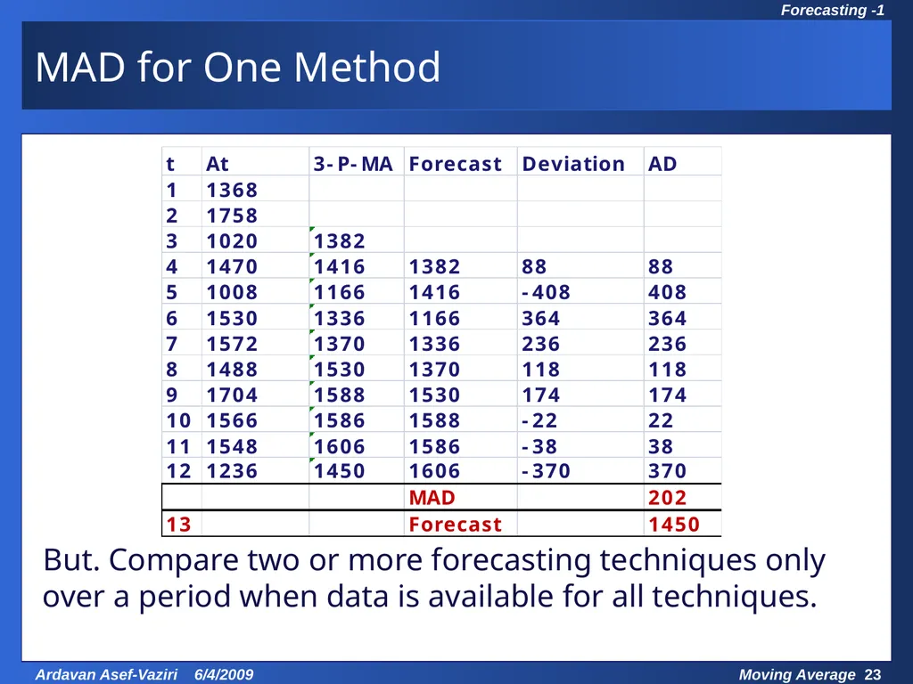
slide23. MAD for One Method But. Compare two or more forecasting techniques only over a period when data is available for all techniques.<br>
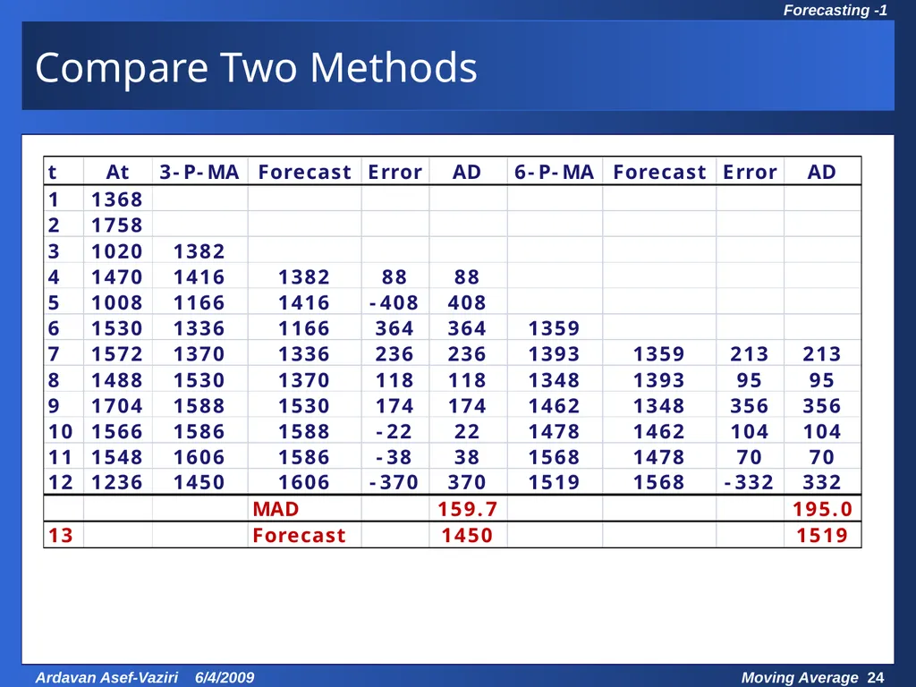
slide24. Compare Two Methods<br>
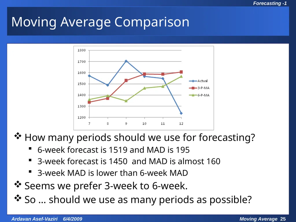
slide25. Moving Average Comparison How many periods should we use for forecasting?
6-week forecast is 1519 and MAD is 195
3-week forecast is 1450 and MAD is almost 160
3-week MAD is lower than 6-week MAD
Seems we prefer 3-week to 6-week.
So … should we use as many periods as possible?<br>
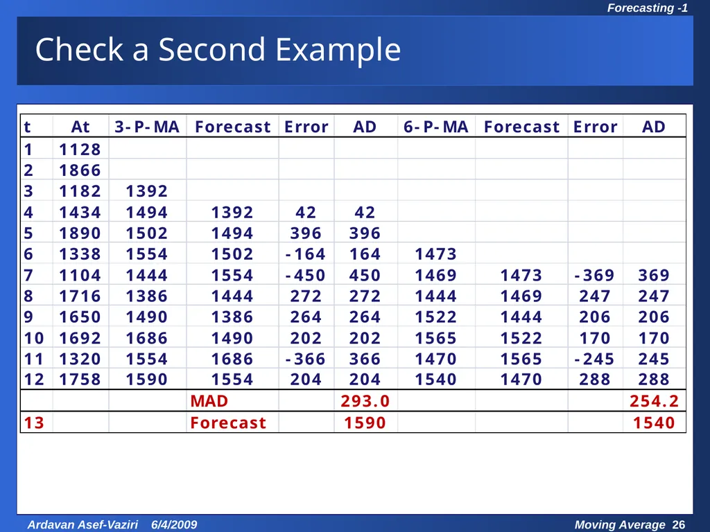
slide26. Check a Second Example<br>
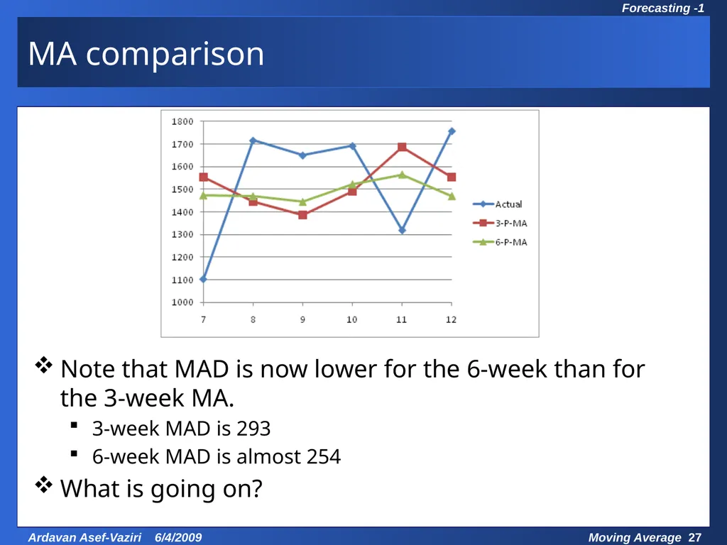
slide27. MA comparison Note that MAD is now lower for the 6-week than for the 3-week MA.
3-week MAD is 293
6-week MAD is almost 254
What is going on?<br>
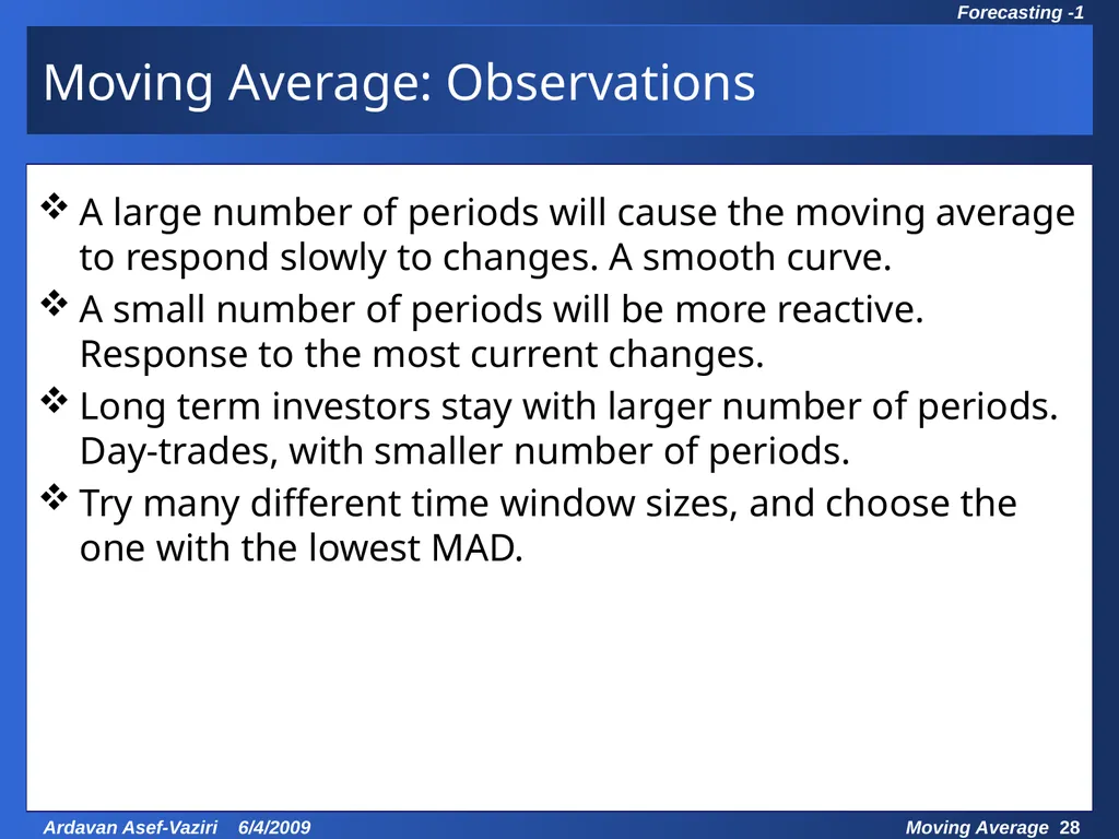
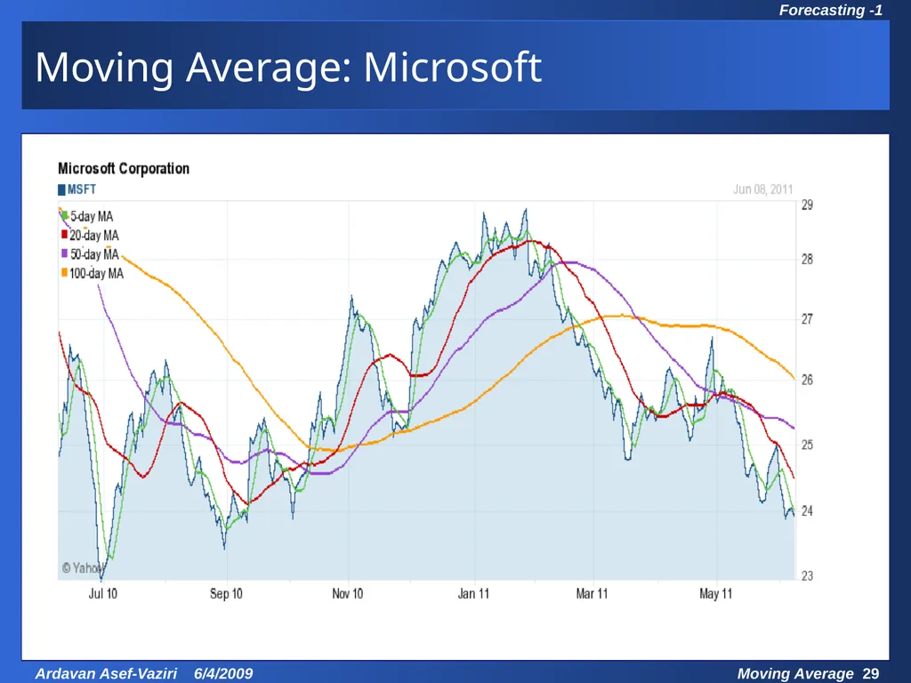
slide28. Moving Average: Observations A large number of periods will cause the moving average to respond slowly to changes. A smooth curve.
A small number of periods will be more reactive. Response to the most current changes.
Long term investors stay with larger number of periods. Day-trades, with smaller number of periods.
Try many different time window sizes, and choose the one with the lowest MAD.<br>
slide29. Moving Average: Microsoft<br>
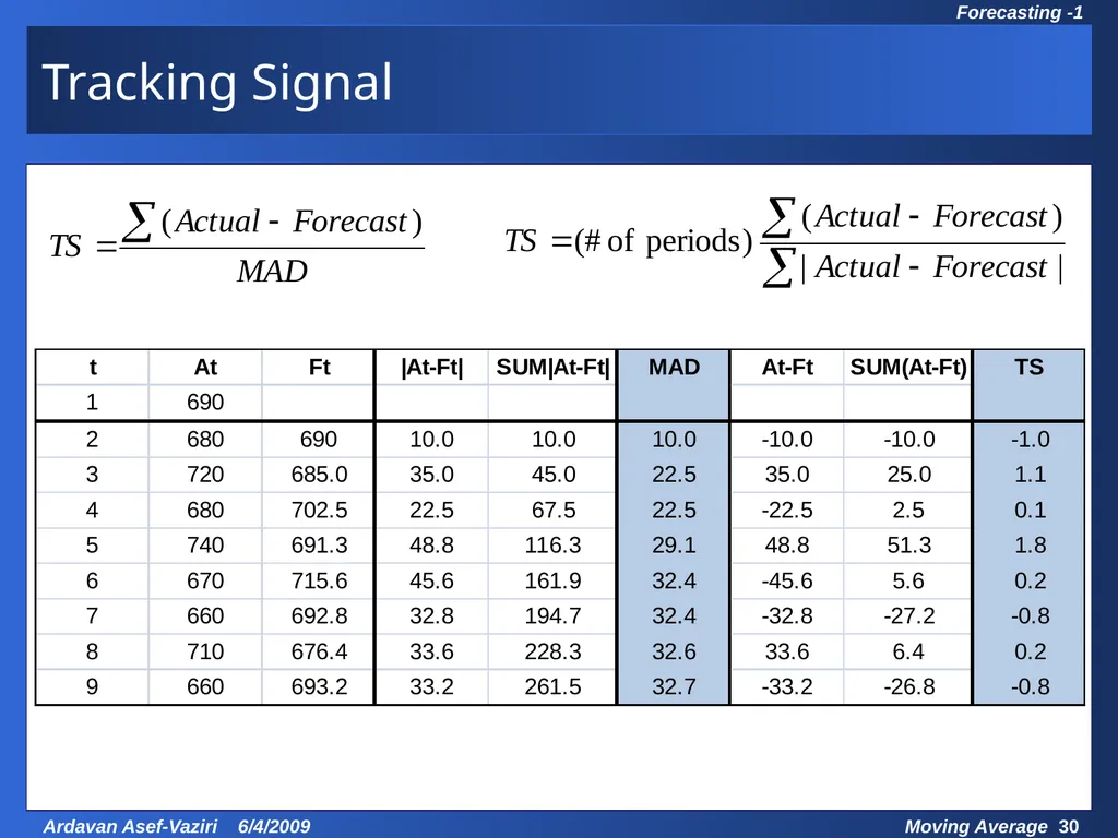
slide30. Tracking Signal<br>
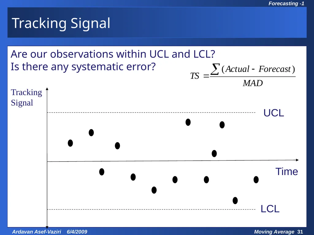
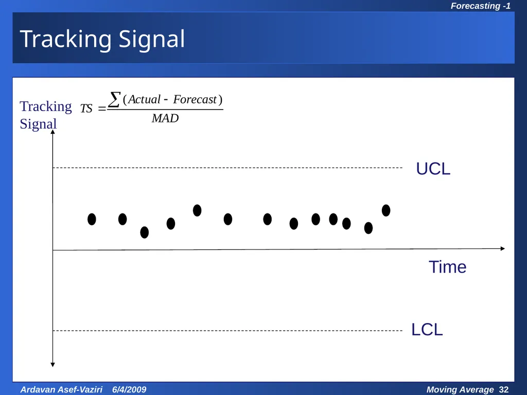
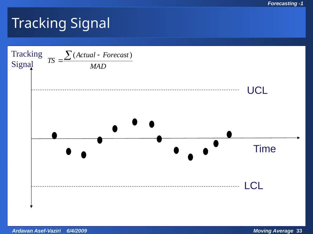
slide31. Tracking Signal Tracking Signal UCL LCL Time Are our observations within UCL and LCL?
Is there any systematic error?<br>
slide32. UCL LCL Time Tracking Signal Tracking Signal<br>
slide33. UCL LCL Time Tracking Signal Tracking Signal<br>
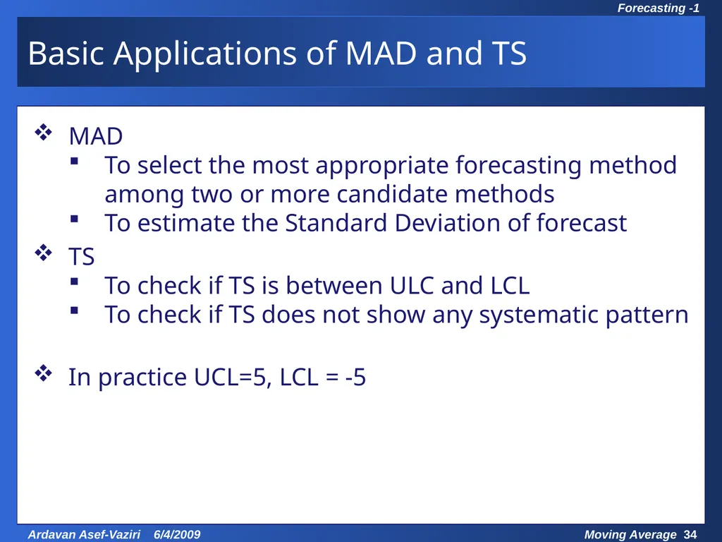
slide34. Basic Applications of MAD and TS MAD
To select the most appropriate forecasting method among two or more candidate methods
To estimate the Standard Deviation of forecast
TS
To check if TS is between ULC and LCL
To check if TS does not show any systematic pattern
In practice UCL=5, LCL = -5<br>
slide35. Chapter 7 Demand Forecasting in a Supply Chain Predictions are usually difficult, especially about the future.
Yogi Berra
The former New York Yankees Catcher<br>
Moving Average
Ardavan Asef-Vaziri
Based on
Operations management: Stevenson
Operations Management: Jacobs, Chase, and Aquilano
Supply Chain Management: Chopra and Meindl
USC Marshall School of Business Lecture Notes
“Those who do not remember the past are condemned to repeat it”
George Santayana Spanish philosopher, essayist, poet and novelist (1863-1952)<br>
slide2. Recoded Lecture on Moving Average Slides https://www.youtube.com/watch?v=gt-YOLxJqBk&t=8s<br>
slide3. Uses of Forecasts Forecast: a prediction of the future value of a variable of interest, such as demand.<br>
slide4. Types of Forecasting Qualitative Techniques
Delphi
Quantitative Techniques
Time Series Analysis - Analyzing data by time periods to determine if trends or patterns exist.
Moving Average
Exponential Smoothing
Causal Relationship Forecasting - Relating demand to an underlying factor other than time.
Linear - Single and Multi Variables
Nonlinear - Single and Multi Variables
Measures of Accuracy
Mean Absolute Deviation, Tracking Signal<br>
slide5. Four Characteristics of Forecasts Forecasts are usually (always) inaccurate (wrong).
Forecasts should be accompanied by a measure of forecast error.
Forecasts for aggregate items are more accurate than individual forecasts. Aggregate forecasts reduce the amount of variability – relative to the aggregate mean demand. Standard Deviation of sum of two variables is less than sum of the Standard Deviation of the two variables.
Long-range forecasts are less accurate than short-range forecasts. Forecasts further into the future tends to be less accurate than those of more imminent events. As time passes, we get better information, and make better prediction.<br>
slide6. Container Handling 2007: World Total 450 MTEUs<br>
slide7. San Pedro Bay (SPB) Ports- Portsts of LA/LB More than 50% of containers coming to US pass through SPB ports. More than 1/3 of the containerized product consumed in all other states pass through SPB ports.
The total value of trade using the southern California trade infrastructure network is around $300 billion, creating around $30 billion in state and local taxes and around 3 million jobs or full time equivalents.
SPB ports need to retain their competing edges.<br>
slide8. US-China Alternative Routes Narvik, Norway Vostochny, Russia Hong Kong, China Singapore Rotterdam, Netherlands Savannah Norfolk New York Prince Rupert, Canada Savannah Norfolk New York Los Angeles Colima, Mexico Ensenada, Mexico<br>
slide9. Competing Edges of SPB Ports Deep-water facilities for 8,000+ container ships.
State-of-the-art on-dock facilities between ship and train.
Intermodal transfer – Ship-train-truck.
Consolidation and distribution facilities for trans-loading- from 20’ and 40’ to 56’.
The last two Characteristics of all Forecasting Techniques<br>
slide10. Strategic Positioning and Smooth Flow<br>
slide11. Strategic Positioning and Smooth Flow<br>
slide12. Qualitative Methods - Delphi Non-quantitative forecasting techniques based on expert opinions and intuition. Typically used when there are no data available.
Delphi Method
Subjective, judgmental
Based on intuition, estimates, and opinions
Expert Opinions
Market Research
Historical Analogies<br>
slide13. Find a relationship between demand and time. Demand Time Time Series Forecasts<br>
slide14. Components of an Observation Observed variable (O) =
Systematic component (S) + Random component (R) Level (current deseasonalized ) Trend (growth or decline) Seasonality (predictable seasonal fluctuation) Systematic component: Expected value of the variable
Random component: The part of the forecast that deviates from the systematic component
Forecast error: difference between forecast and actual demand<br>
slide15. Naive Forecast
Moving Average
Exponential Smoothing Time Series Techniques<br>
slide16. We sold 250 wheels last week....
Now, next week we should sell.… At : Actual demand in period t F(t+1) : Forecast of demand for period t+1 F(t+1) = At Naive Forecast 250 wheels The naive forecast can also serve as an
accuracy standard for other techniques.<br>
slide17. Moving Average Three period moving average in period 7 is the average of: MAt10 = (At+ At-1+ At-2 +At-3+ ….+ At-9 )/10 MA73 = (A7+ A6+ A5 )/3 Three period moving average in period t is the average of: MAt3 = (At+ At-1+ At-2 )/3 Ten period moving average in period t is the average of:<br>
slide18. Forecast Using Moving Average Forecast for period t+1 is equal to moving average for period t Ft+1 =MAtn n period moving average in period t is the average of: MAtn = (At+ At-1+ At-2 +At-3+ ….+ At-n+1 )/n Ft+1 =MAtn = (At+ At-1+ At-2 +At-3+ ….+ At-n+1 )/n<br>
slide19. An example for comparison of two Moving Averages Let’s develop 3-week and 6-week moving average forecasts for demand in week 13.<br>
slide20. 3-Period and 6-Period Moving Average<br>
slide21. MAD to Compare Two or More Methods<br>
slide22. How do we measure errors? Standard Deviation of Error = 1.25MAD Error is assumed to be normally distributed
A MEAN (AVERAGE) = 0
STANDARD DEVIATION = 1.25MAD
Therefore, our forecast is also normally distributed
A MEAN (AVERAGE) = Ft
STANDARD DEVIATION = 1.25MAD Error = At - Ft<br>
slide23. MAD for One Method But. Compare two or more forecasting techniques only over a period when data is available for all techniques.<br>
slide24. Compare Two Methods<br>
slide25. Moving Average Comparison How many periods should we use for forecasting?
6-week forecast is 1519 and MAD is 195
3-week forecast is 1450 and MAD is almost 160
3-week MAD is lower than 6-week MAD
Seems we prefer 3-week to 6-week.
So … should we use as many periods as possible?<br>
slide26. Check a Second Example<br>
slide27. MA comparison Note that MAD is now lower for the 6-week than for the 3-week MA.
3-week MAD is 293
6-week MAD is almost 254
What is going on?<br>
slide28. Moving Average: Observations A large number of periods will cause the moving average to respond slowly to changes. A smooth curve.
A small number of periods will be more reactive. Response to the most current changes.
Long term investors stay with larger number of periods. Day-trades, with smaller number of periods.
Try many different time window sizes, and choose the one with the lowest MAD.<br>
slide29. Moving Average: Microsoft<br>
slide30. Tracking Signal<br>
slide31. Tracking Signal Tracking Signal UCL LCL Time Are our observations within UCL and LCL?
Is there any systematic error?<br>
slide32. UCL LCL Time Tracking Signal Tracking Signal<br>
slide33. UCL LCL Time Tracking Signal Tracking Signal<br>
slide34. Basic Applications of MAD and TS MAD
To select the most appropriate forecasting method among two or more candidate methods
To estimate the Standard Deviation of forecast
TS
To check if TS is between ULC and LCL
To check if TS does not show any systematic pattern
In practice UCL=5, LCL = -5<br>
slide35. Chapter 7 Demand Forecasting in a Supply Chain Predictions are usually difficult, especially about the future.
Yogi Berra
The former New York Yankees Catcher<br>