
Chapter 9 Structural Equation Modeling: An
Description: Chapter 9 Structural Equation Modeling: An Introduction Section V Moving Beyond the Basics For use with Hair, Black, Babin and Anderson, Multivariate Data Analysis 8e 2018 Cengage Learning EMEA Chapter 9: Structural Equations Modeling
Related Topics
Download Presentation
"Chapter 9 Structural Equation Modeling: An" is the property of its rightful owner. Permission is granted to download and print the materials on this website for personal, non-commercial use only, and to display it on your personal computer provided you do not modify the materials and that you retain all copyright notices contained in the materials. By downloading content from our website, you accept the terms of this agreement.
Presentation Transcript
slide1. Chapter 9
Structural Equation Modeling: An Introduction Section V
Moving Beyond the Basics For use with Hair, Black, Babin and Anderson, Multivariate Data Analysis 8e © 2018 Cengage Learning EMEA<br>
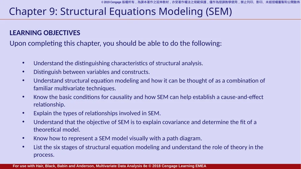
slide2. Chapter 9: Structural Equations Modeling (SEM) LEARNING OBJECTIVES
Upon completing this chapter, you should be able to do the following:
Understand the distinguishing characteristics of structural analysis.
Distinguish between variables and constructs.
Understand structural equation modeling and how it can be thought of as a combination of familiar multivariate techniques.
Know the basic conditions for causality and how SEM can help establish a cause-and-effect relationship.
Explain the types of relationships involved in SEM.
Understand that the objective of SEM is to explain covariance and determine the fit of a theoretical model.
Know how to represent a SEM model visually with a path diagram.
List the six stages of structural equation modeling and understand the role of theory in the process. For use with Hair, Black, Babin and Anderson, Multivariate Data Analysis 8e © 2018 Cengage Learning EMEA<br>
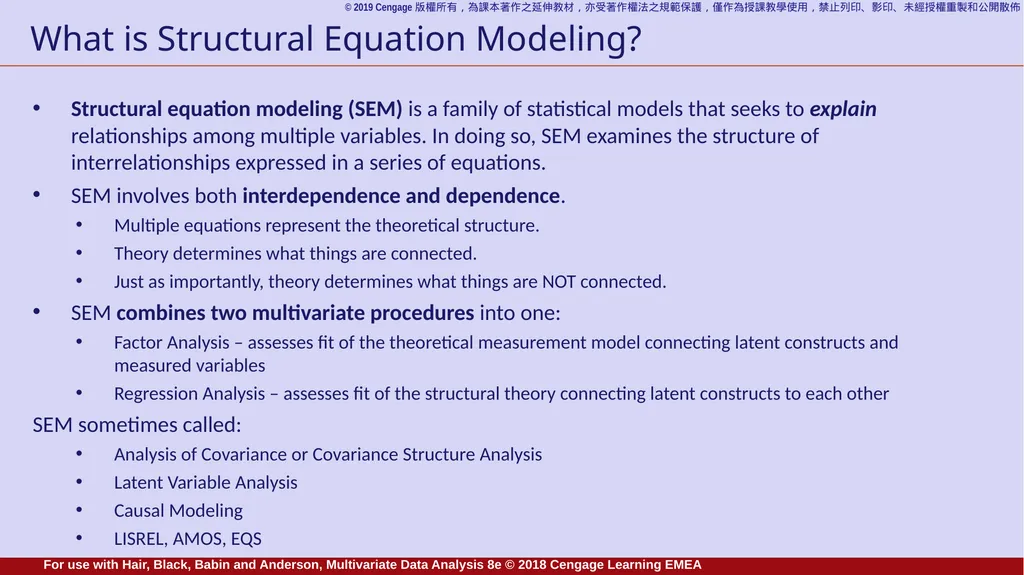
slide3. What is Structural Equation Modeling? Structural equation modeling (SEM) is a family of statistical models that seeks to explain relationships among multiple variables. In doing so, SEM examines the structure of interrelationships expressed in a series of equations.
SEM involves both interdependence and dependence.
Multiple equations represent the theoretical structure.
Theory determines what things are connected.
Just as importantly, theory determines what things are NOT connected.
SEM combines two multivariate procedures into one:
Factor Analysis – assesses fit of the theoretical measurement model connecting latent constructs and measured variables
Regression Analysis – assesses fit of the structural theory connecting latent constructs to each other
SEM sometimes called:
Analysis of Covariance or Covariance Structure Analysis
Latent Variable Analysis
Causal Modeling
LISREL, AMOS, EQS For use with Hair, Black, Babin and Anderson, Multivariate Data Analysis 8e © 2018 Cengage Learning EMEA<br>
slide4. Notes on the Structure in SEM Structure Represents Theory
The user specifies a structural model that includes a limited set of relationships. Thus, SEM is distinct from other multivariate procedures:
Structural analysis is not exploratory
SEM tests the user’s theory and does not explore relationships or reveal a model
SEM provides more accurate estimates of parameters
Corrects for error attenuation (suggests what the relationship would be if no unreliability existed)
Structural equations only include the relationships necessary to represent the model.
All other possible connections are assumed to be 0 (do not exist)
Structural equations are contrasted with reduced form equations:
A reduced form equation solves for a single endogenous construct (or dependent variable) in a single equation with all and only exogenous constructs (independent variables) employed as predictors For use with Hair, Black, Babin and Anderson, Multivariate Data Analysis 8e © 2018 Cengage Learning EMEA<br>
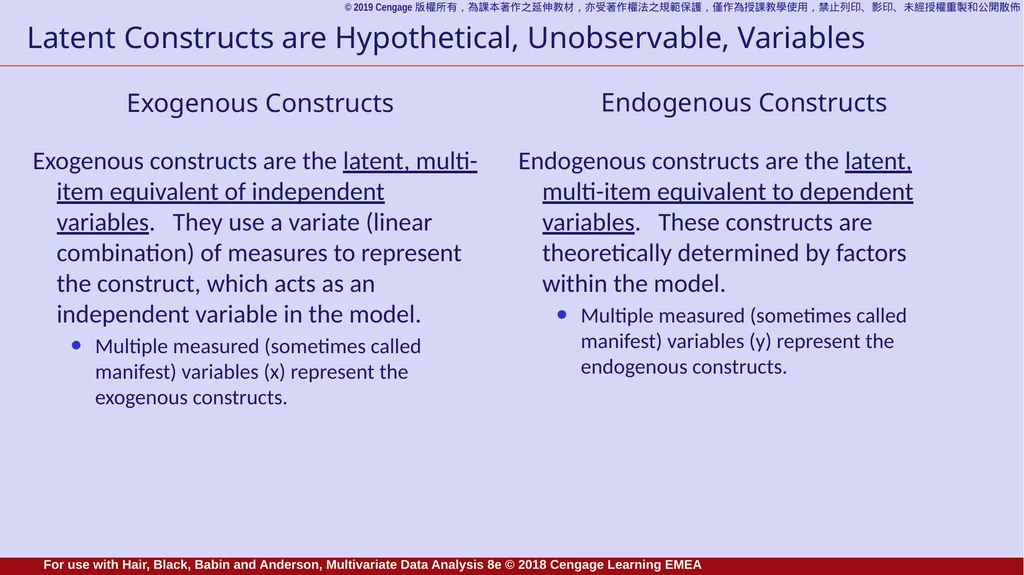
slide5. Latent Constructs are Hypothetical, Unobservable, Variables Exogenous constructs are the latent, multi-item equivalent of independent variables. They use a variate (linear combination) of measures to represent the construct, which acts as an independent variable in the model.
Multiple measured (sometimes called manifest) variables (x) represent the exogenous constructs. Endogenous constructs are the latent, multi-item equivalent to dependent variables. These constructs are theoretically determined by factors within the model.
Multiple measured (sometimes called manifest) variables (y) represent the endogenous constructs. Exogenous Constructs Endogenous Constructs For use with Hair, Black, Babin and Anderson, Multivariate Data Analysis 8e © 2018 Cengage Learning EMEA<br>
slide6. Defining a Model SEM tests models
A model is a representation of a theory.
A theory is a systematic set of relationships providing a consistent and comprehensive explanation of phenomena. SEM involves:
Measurement theory – provides measurement model defining pattern (correspondence rules) of relationships between measured variables and each latent construct
Structural theory – provides correspondence rules linking constructs to each other For use with Hair, Black, Babin and Anderson, Multivariate Data Analysis 8e © 2018 Cengage Learning EMEA<br>
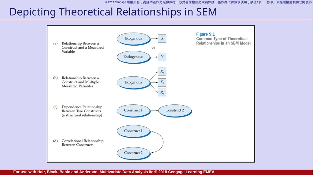
slide7. Depicting Theoretical Relationships in SEM For use with Hair, Black, Babin and Anderson, Multivariate Data Analysis 8e © 2018 Cengage Learning EMEA<br>
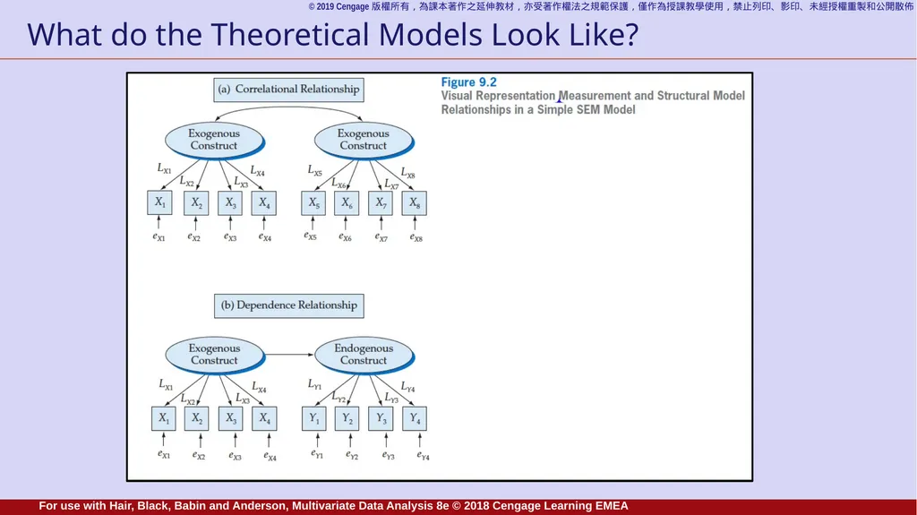
slide8. What do the Theoretical Models Look Like? For use with Hair, Black, Babin and Anderson, Multivariate Data Analysis 8e © 2018 Cengage Learning EMEA<br>
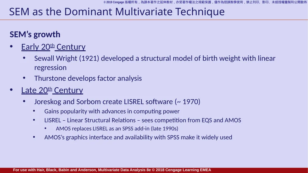
slide9. SEM as the Dominant Multivariate Technique SEM’s growth
Early 20th Century
Sewall Wright (1921) developed a structural model of birth weight with linear regression
Thurstone develops factor analysis
Late 20th Century
Joreskog and Sorbom create LISREL software (~ 1970)
Gains popularity with advances in computing power
LISREL – Linear Structural Relations – sees competition from EQS and AMOS
AMOS replaces LISREL as an SPSS add-in (late 1990s)
AMOS’s graphics interface and availability with SPSS make it widely used For use with Hair, Black, Babin and Anderson, Multivariate Data Analysis 8e © 2018 Cengage Learning EMEA<br>
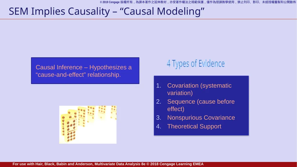
slide10. SEM Implies Causality – “Causal Modeling” Causal Inference – Hypothesizes a “cause-and-effect” relationship. Covariation (systematic variation)
Sequence (cause before effect)
Nonspurious Covariance
Theoretical Support 4 Types of Evidence For use with Hair, Black, Babin and Anderson, Multivariate Data Analysis 8e © 2018 Cengage Learning EMEA<br>
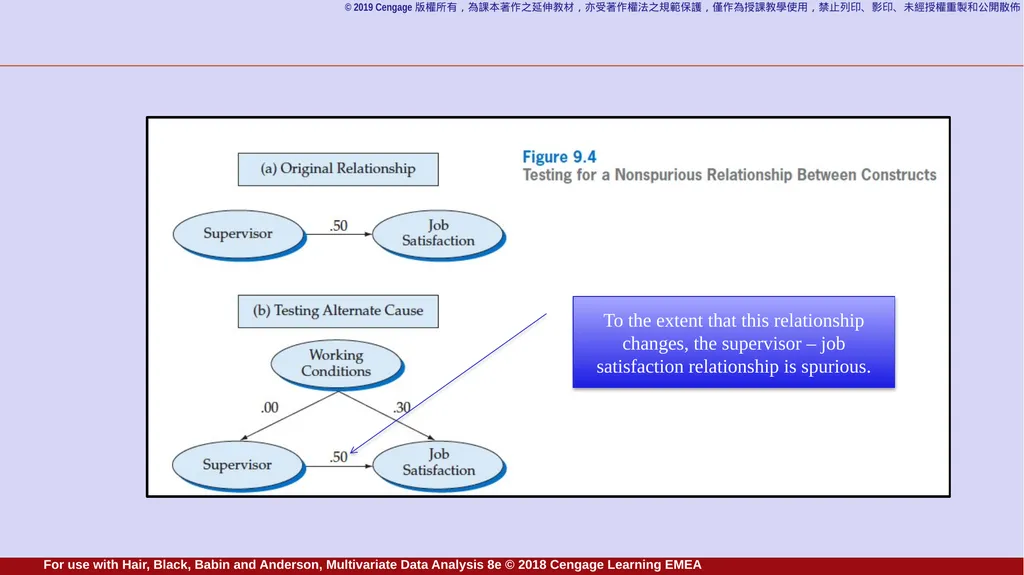
slide11. To the extent that this relationship changes, the supervisor – job satisfaction relationship is spurious. For use with Hair, Black, Babin and Anderson, Multivariate Data Analysis 8e © 2018 Cengage Learning EMEA<br>
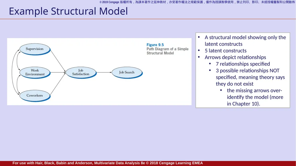
slide12. Example Structural Model A structural model showing only the latent constructs
5 latent constructs
Arrows depict relationships
7 relationships specified
3 possible relationships NOT specified, meaning theory says they do not exist
the missing arrows over-identify the model (more in Chapter 10). For use with Hair, Black, Babin and Anderson, Multivariate Data Analysis 8e © 2018 Cengage Learning EMEA<br>
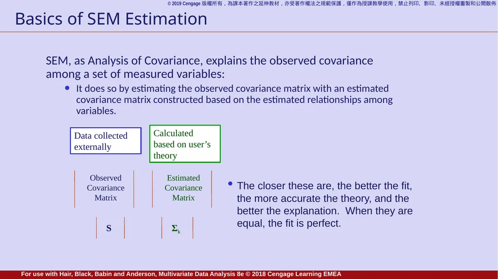
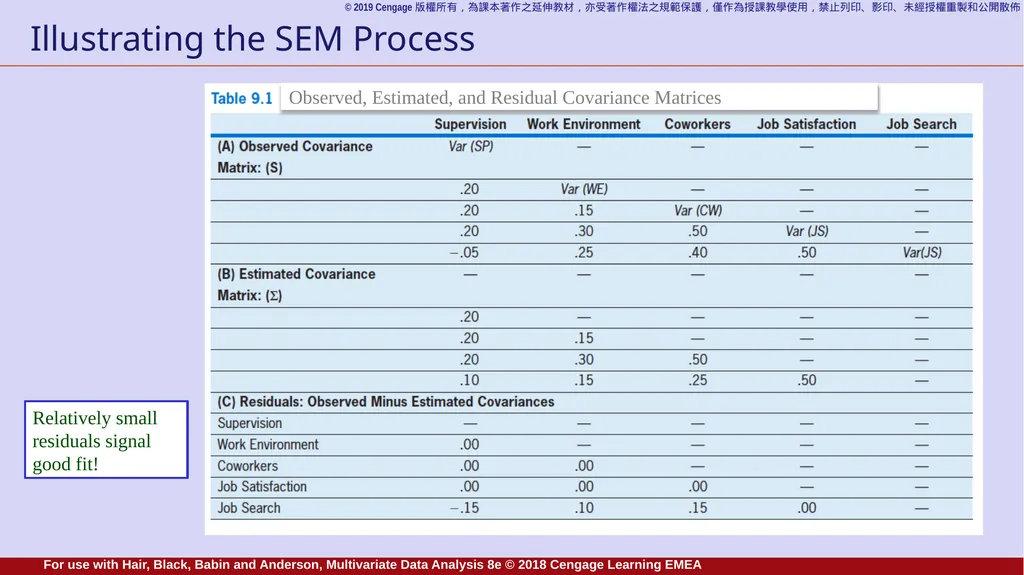
slide13. Basics of SEM Estimation SEM, as Analysis of Covariance, explains the observed covariance among a set of measured variables:
It does so by estimating the observed covariance matrix with an estimated covariance matrix constructed based on the estimated relationships among variables. The closer these are, the better the fit, the more accurate the theory, and the better the explanation. When they are equal, the fit is perfect. Calculated based on user’s theory Data collected externally For use with Hair, Black, Babin and Anderson, Multivariate Data Analysis 8e © 2018 Cengage Learning EMEA<br>
slide14. Illustrating the SEM Process Relatively small residuals signal good fit! Observed, Estimated, and Residual Covariance Matrices For use with Hair, Black, Babin and Anderson, Multivariate Data Analysis 8e © 2018 Cengage Learning EMEA<br>
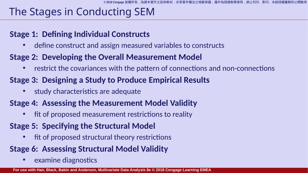
slide15. The Stages in Conducting SEM Stage 1: Defining Individual Constructs
define construct and assign measured variables to constructs
Stage 2: Developing the Overall Measurement Model
restrict the covariances with the pattern of connections and non-connections
Stage 3: Designing a Study to Produce Empirical Results
study characteristics are adequate
Stage 4: Assessing the Measurement Model Validity
fit of proposed measurement restrictions to reality
Stage 5: Specifying the Structural Model
fit of proposed structural theory restrictions
Stage 6: Assessing Structural Model Validity
examine diagnostics For use with Hair, Black, Babin and Anderson, Multivariate Data Analysis 8e © 2018 Cengage Learning EMEA<br>
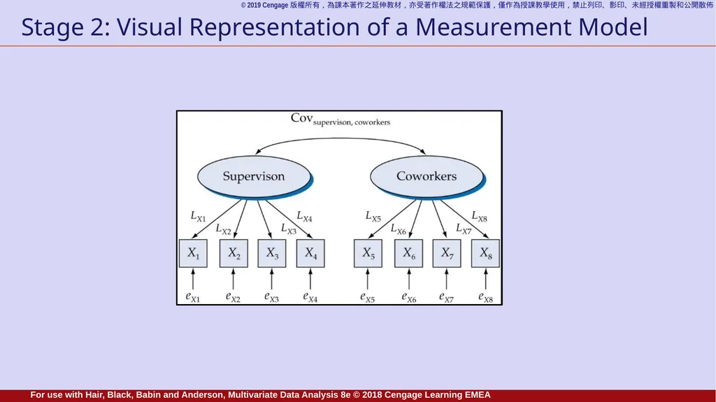
slide16. Stage 2: Visual Representation of a Measurement Model For use with Hair, Black, Babin and Anderson, Multivariate Data Analysis 8e © 2018 Cengage Learning EMEA<br>
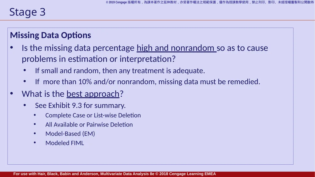
slide17. Stage 3 Missing Data Options
Is the missing data percentage high and nonrandom so as to cause problems in estimation or interpretation?
If small and random, then any treatment is adequate.
If more than 10% and/or nonrandom, missing data must be remedied.
What is the best approach?
See Exhibit 9.3 for summary.
Complete Case or List-wise Deletion
All Available or Pairwise Deletion
Model-Based (EM)
Modeled FIML For use with Hair, Black, Babin and Anderson, Multivariate Data Analysis 8e © 2018 Cengage Learning EMEA<br>
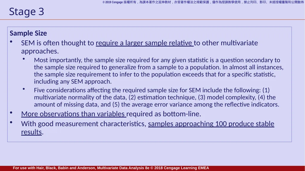
slide18. Stage 3 Sample Size
SEM is often thought to require a larger sample relative to other multivariate approaches.
Most importantly, the sample size required for any given statistic is a question secondary to the sample size required to generalize from a sample to a population. In almost all instances, the sample size requirement to infer to the population exceeds that for a specific statistic, including any SEM approach.
Five considerations affecting the required sample size for SEM include the following: (1) multivariate normality of the data, (2) estimation technique, (3) model complexity, (4) the amount of missing data, and (5) the average error variance among the reflective indicators.
More observations than variables required as bottom-line.
With good measurement characteristics, samples approaching 100 produce stable results. For use with Hair, Black, Babin and Anderson, Multivariate Data Analysis 8e © 2018 Cengage Learning EMEA<br>
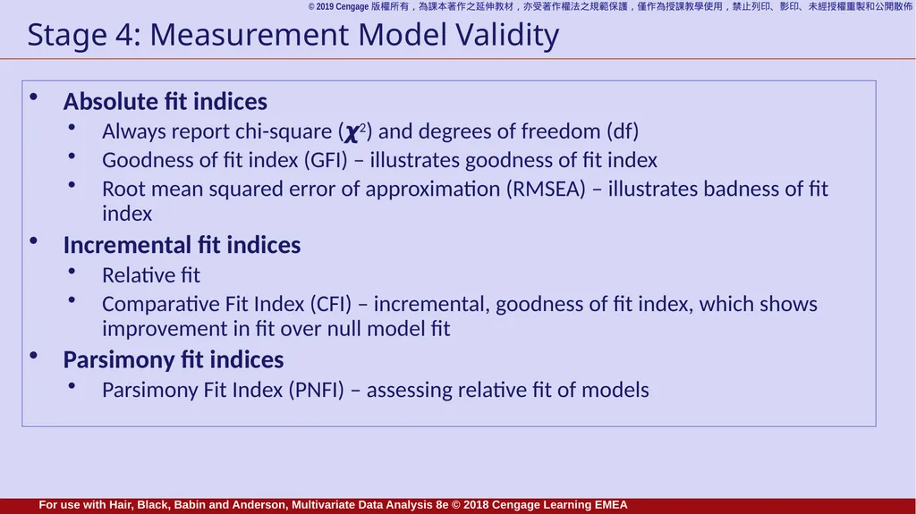
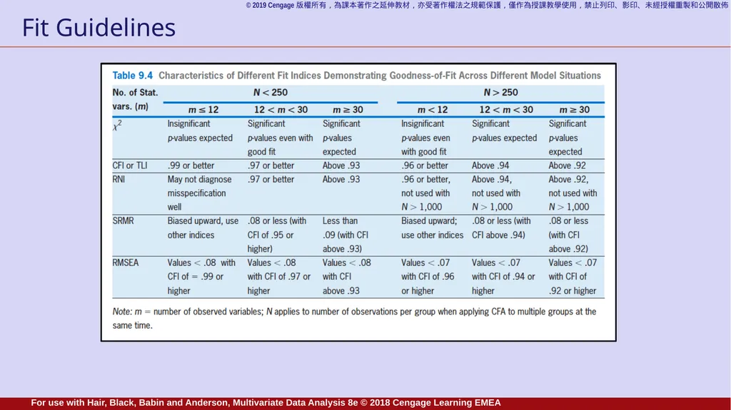
slide19. Stage 4: Measurement Model Validity Absolute fit indices
Always report chi-square (𝟀2) and degrees of freedom (df)
Goodness of fit index (GFI) – illustrates goodness of fit index
Root mean squared error of approximation (RMSEA) – illustrates badness of fit index
Incremental fit indices
Relative fit
Comparative Fit Index (CFI) – incremental, goodness of fit index, which shows improvement in fit over null model fit
Parsimony fit indices
Parsimony Fit Index (PNFI) – assessing relative fit of models For use with Hair, Black, Babin and Anderson, Multivariate Data Analysis 8e © 2018 Cengage Learning EMEA<br>
slide20. Fit Guidelines For use with Hair, Black, Babin and Anderson, Multivariate Data Analysis 8e © 2018 Cengage Learning EMEA<br>
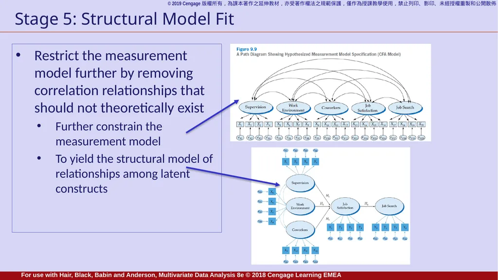
slide21. Stage 5: Structural Model Fit Restrict the measurement model further by removing correlation relationships that should not theoretically exist
Further constrain the measurement model
To yield the structural model of relationships among latent constructs For use with Hair, Black, Babin and Anderson, Multivariate Data Analysis 8e © 2018 Cengage Learning EMEA<br>
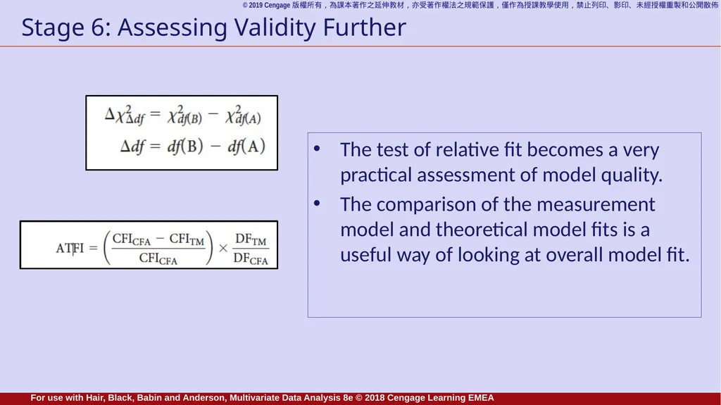
slide22. Stage 6: Assessing Validity Further The test of relative fit becomes a very practical assessment of model quality.
The comparison of the measurement model and theoretical model fits is a useful way of looking at overall model fit. For use with Hair, Black, Babin and Anderson, Multivariate Data Analysis 8e © 2018 Cengage Learning EMEA<br>
slide23. Learning Checkpoints Provide a basic overview of “what is SEM?”
How does SEM combines factor analysis and linear regression?
Why is SEM very appropriate for analyzing latent constructs?
What are the conditions of causality?
What is the purpose of reproducing the covariance matrix by representing the user’s theory with equations?
List the stages of a complete SEM analysis. For use with Hair, Black, Babin and Anderson, Multivariate Data Analysis 8e © 2018 Cengage Learning EMEA<br>
Moving Beyond the Basics For use with Hair, Black, Babin and Anderson, Multivariate Data Analysis 8e © 2018 Cengage Learning EMEA<br>
slide2. Chapter 9: Structural Equations Modeling (SEM) LEARNING OBJECTIVES
Upon completing this chapter, you should be able to do the following:
Understand the distinguishing characteristics of structural analysis.
Distinguish between variables and constructs.
Understand structural equation modeling and how it can be thought of as a combination of familiar multivariate techniques.
Know the basic conditions for causality and how SEM can help establish a cause-and-effect relationship.
Explain the types of relationships involved in SEM.
Understand that the objective of SEM is to explain covariance and determine the fit of a theoretical model.
Know how to represent a SEM model visually with a path diagram.
List the six stages of structural equation modeling and understand the role of theory in the process. For use with Hair, Black, Babin and Anderson, Multivariate Data Analysis 8e © 2018 Cengage Learning EMEA<br>
slide3. What is Structural Equation Modeling? Structural equation modeling (SEM) is a family of statistical models that seeks to explain relationships among multiple variables. In doing so, SEM examines the structure of interrelationships expressed in a series of equations.
SEM involves both interdependence and dependence.
Multiple equations represent the theoretical structure.
Theory determines what things are connected.
Just as importantly, theory determines what things are NOT connected.
SEM combines two multivariate procedures into one:
Factor Analysis – assesses fit of the theoretical measurement model connecting latent constructs and measured variables
Regression Analysis – assesses fit of the structural theory connecting latent constructs to each other
SEM sometimes called:
Analysis of Covariance or Covariance Structure Analysis
Latent Variable Analysis
Causal Modeling
LISREL, AMOS, EQS For use with Hair, Black, Babin and Anderson, Multivariate Data Analysis 8e © 2018 Cengage Learning EMEA<br>
slide4. Notes on the Structure in SEM Structure Represents Theory
The user specifies a structural model that includes a limited set of relationships. Thus, SEM is distinct from other multivariate procedures:
Structural analysis is not exploratory
SEM tests the user’s theory and does not explore relationships or reveal a model
SEM provides more accurate estimates of parameters
Corrects for error attenuation (suggests what the relationship would be if no unreliability existed)
Structural equations only include the relationships necessary to represent the model.
All other possible connections are assumed to be 0 (do not exist)
Structural equations are contrasted with reduced form equations:
A reduced form equation solves for a single endogenous construct (or dependent variable) in a single equation with all and only exogenous constructs (independent variables) employed as predictors For use with Hair, Black, Babin and Anderson, Multivariate Data Analysis 8e © 2018 Cengage Learning EMEA<br>
slide5. Latent Constructs are Hypothetical, Unobservable, Variables Exogenous constructs are the latent, multi-item equivalent of independent variables. They use a variate (linear combination) of measures to represent the construct, which acts as an independent variable in the model.
Multiple measured (sometimes called manifest) variables (x) represent the exogenous constructs. Endogenous constructs are the latent, multi-item equivalent to dependent variables. These constructs are theoretically determined by factors within the model.
Multiple measured (sometimes called manifest) variables (y) represent the endogenous constructs. Exogenous Constructs Endogenous Constructs For use with Hair, Black, Babin and Anderson, Multivariate Data Analysis 8e © 2018 Cengage Learning EMEA<br>
slide6. Defining a Model SEM tests models
A model is a representation of a theory.
A theory is a systematic set of relationships providing a consistent and comprehensive explanation of phenomena. SEM involves:
Measurement theory – provides measurement model defining pattern (correspondence rules) of relationships between measured variables and each latent construct
Structural theory – provides correspondence rules linking constructs to each other For use with Hair, Black, Babin and Anderson, Multivariate Data Analysis 8e © 2018 Cengage Learning EMEA<br>
slide7. Depicting Theoretical Relationships in SEM For use with Hair, Black, Babin and Anderson, Multivariate Data Analysis 8e © 2018 Cengage Learning EMEA<br>
slide8. What do the Theoretical Models Look Like? For use with Hair, Black, Babin and Anderson, Multivariate Data Analysis 8e © 2018 Cengage Learning EMEA<br>
slide9. SEM as the Dominant Multivariate Technique SEM’s growth
Early 20th Century
Sewall Wright (1921) developed a structural model of birth weight with linear regression
Thurstone develops factor analysis
Late 20th Century
Joreskog and Sorbom create LISREL software (~ 1970)
Gains popularity with advances in computing power
LISREL – Linear Structural Relations – sees competition from EQS and AMOS
AMOS replaces LISREL as an SPSS add-in (late 1990s)
AMOS’s graphics interface and availability with SPSS make it widely used For use with Hair, Black, Babin and Anderson, Multivariate Data Analysis 8e © 2018 Cengage Learning EMEA<br>
slide10. SEM Implies Causality – “Causal Modeling” Causal Inference – Hypothesizes a “cause-and-effect” relationship. Covariation (systematic variation)
Sequence (cause before effect)
Nonspurious Covariance
Theoretical Support 4 Types of Evidence For use with Hair, Black, Babin and Anderson, Multivariate Data Analysis 8e © 2018 Cengage Learning EMEA<br>
slide11. To the extent that this relationship changes, the supervisor – job satisfaction relationship is spurious. For use with Hair, Black, Babin and Anderson, Multivariate Data Analysis 8e © 2018 Cengage Learning EMEA<br>
slide12. Example Structural Model A structural model showing only the latent constructs
5 latent constructs
Arrows depict relationships
7 relationships specified
3 possible relationships NOT specified, meaning theory says they do not exist
the missing arrows over-identify the model (more in Chapter 10). For use with Hair, Black, Babin and Anderson, Multivariate Data Analysis 8e © 2018 Cengage Learning EMEA<br>
slide13. Basics of SEM Estimation SEM, as Analysis of Covariance, explains the observed covariance among a set of measured variables:
It does so by estimating the observed covariance matrix with an estimated covariance matrix constructed based on the estimated relationships among variables. The closer these are, the better the fit, the more accurate the theory, and the better the explanation. When they are equal, the fit is perfect. Calculated based on user’s theory Data collected externally For use with Hair, Black, Babin and Anderson, Multivariate Data Analysis 8e © 2018 Cengage Learning EMEA<br>
slide14. Illustrating the SEM Process Relatively small residuals signal good fit! Observed, Estimated, and Residual Covariance Matrices For use with Hair, Black, Babin and Anderson, Multivariate Data Analysis 8e © 2018 Cengage Learning EMEA<br>
slide15. The Stages in Conducting SEM Stage 1: Defining Individual Constructs
define construct and assign measured variables to constructs
Stage 2: Developing the Overall Measurement Model
restrict the covariances with the pattern of connections and non-connections
Stage 3: Designing a Study to Produce Empirical Results
study characteristics are adequate
Stage 4: Assessing the Measurement Model Validity
fit of proposed measurement restrictions to reality
Stage 5: Specifying the Structural Model
fit of proposed structural theory restrictions
Stage 6: Assessing Structural Model Validity
examine diagnostics For use with Hair, Black, Babin and Anderson, Multivariate Data Analysis 8e © 2018 Cengage Learning EMEA<br>
slide16. Stage 2: Visual Representation of a Measurement Model For use with Hair, Black, Babin and Anderson, Multivariate Data Analysis 8e © 2018 Cengage Learning EMEA<br>
slide17. Stage 3 Missing Data Options
Is the missing data percentage high and nonrandom so as to cause problems in estimation or interpretation?
If small and random, then any treatment is adequate.
If more than 10% and/or nonrandom, missing data must be remedied.
What is the best approach?
See Exhibit 9.3 for summary.
Complete Case or List-wise Deletion
All Available or Pairwise Deletion
Model-Based (EM)
Modeled FIML For use with Hair, Black, Babin and Anderson, Multivariate Data Analysis 8e © 2018 Cengage Learning EMEA<br>
slide18. Stage 3 Sample Size
SEM is often thought to require a larger sample relative to other multivariate approaches.
Most importantly, the sample size required for any given statistic is a question secondary to the sample size required to generalize from a sample to a population. In almost all instances, the sample size requirement to infer to the population exceeds that for a specific statistic, including any SEM approach.
Five considerations affecting the required sample size for SEM include the following: (1) multivariate normality of the data, (2) estimation technique, (3) model complexity, (4) the amount of missing data, and (5) the average error variance among the reflective indicators.
More observations than variables required as bottom-line.
With good measurement characteristics, samples approaching 100 produce stable results. For use with Hair, Black, Babin and Anderson, Multivariate Data Analysis 8e © 2018 Cengage Learning EMEA<br>
slide19. Stage 4: Measurement Model Validity Absolute fit indices
Always report chi-square (𝟀2) and degrees of freedom (df)
Goodness of fit index (GFI) – illustrates goodness of fit index
Root mean squared error of approximation (RMSEA) – illustrates badness of fit index
Incremental fit indices
Relative fit
Comparative Fit Index (CFI) – incremental, goodness of fit index, which shows improvement in fit over null model fit
Parsimony fit indices
Parsimony Fit Index (PNFI) – assessing relative fit of models For use with Hair, Black, Babin and Anderson, Multivariate Data Analysis 8e © 2018 Cengage Learning EMEA<br>
slide20. Fit Guidelines For use with Hair, Black, Babin and Anderson, Multivariate Data Analysis 8e © 2018 Cengage Learning EMEA<br>
slide21. Stage 5: Structural Model Fit Restrict the measurement model further by removing correlation relationships that should not theoretically exist
Further constrain the measurement model
To yield the structural model of relationships among latent constructs For use with Hair, Black, Babin and Anderson, Multivariate Data Analysis 8e © 2018 Cengage Learning EMEA<br>
slide22. Stage 6: Assessing Validity Further The test of relative fit becomes a very practical assessment of model quality.
The comparison of the measurement model and theoretical model fits is a useful way of looking at overall model fit. For use with Hair, Black, Babin and Anderson, Multivariate Data Analysis 8e © 2018 Cengage Learning EMEA<br>
slide23. Learning Checkpoints Provide a basic overview of “what is SEM?”
How does SEM combines factor analysis and linear regression?
Why is SEM very appropriate for analyzing latent constructs?
What are the conditions of causality?
What is the purpose of reproducing the covariance matrix by representing the user’s theory with equations?
List the stages of a complete SEM analysis. For use with Hair, Black, Babin and Anderson, Multivariate Data Analysis 8e © 2018 Cengage Learning EMEA<br>