
Chi-Square Test Karl Pearson introduced Chi-Square
MT
Published · 28 slides · 0 views

1 / 1


Description
Chi-Square Test Karl Pearson introduced Chi-Square (X2) which is a statistical test used to determine whether your experimentally observed results are consistent with your hypothesis. Test statistics measure the agreement between actual
Related Topics
Share
Embed code
Download this presentation From Below
"Chi-Square Test Karl Pearson introduced Chi-Square" is the property of its rightful owner. Permission is granted to download and print the materials on this website for personal, non-commercial use only, and to display it on your personal computer provided you do not modify the materials and that you retain all copyright notices contained in the materials. By downloading content from our website, you accept the terms of this agreement.
Presentation Transcript
01
Chi-Square Test<br>
02
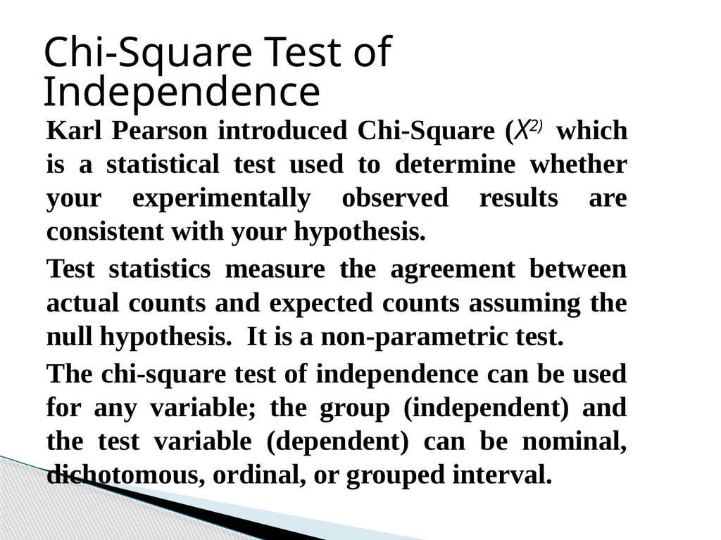
Karl Pearson introduced Chi-Square (X2) which is a statistical test used to determine whether your experimentally observed results are consistent with your hypothesis.
Test statistics measure the agreement between actual counts and expected counts assuming the null hypothesis. It is a non-parametric test.
The chi-square test of independence can be used for any variable; the group (independent) and the test variable (dependent) can be nominal, dichotomous, ordinal, or grouped interval. Chi-Square Test of Independence<br>
Test statistics measure the agreement between actual counts and expected counts assuming the null hypothesis. It is a non-parametric test.
The chi-square test of independence can be used for any variable; the group (independent) and the test variable (dependent) can be nominal, dichotomous, ordinal, or grouped interval. Chi-Square Test of Independence<br>
03
Introduction
Characteristics of the test
Chi-square distribution
Application of Chi square test
Calculation of the Chi square test
Condition for the application of the test
Example
Limitations of the test Chi-square Test<br>
Characteristics of the test
Chi-square distribution
Application of Chi square test
Calculation of the Chi square test
Condition for the application of the test
Example
Limitations of the test Chi-square Test<br>
04
Parametric test- The test in which the population constants like mean, std. deviation, std error, correlation coefficient, proportion etc. and data tend to follow one assumed or established distribution such as normal, binomial, poisson etc.
Non-parametric test- the test in which no constant of a population is used. Data do not follow any specific distribution and no assumption are made in these tests. Eg. To classify goods, better and best, we just allocate arbitrary numbers or marks to each category.
Hypothesis- It is a definite statement about the population parameters. Important terms<br>
Non-parametric test- the test in which no constant of a population is used. Data do not follow any specific distribution and no assumption are made in these tests. Eg. To classify goods, better and best, we just allocate arbitrary numbers or marks to each category.
Hypothesis- It is a definite statement about the population parameters. Important terms<br>
05
H0- states that no association exists between the two cross-tabulated variables in the population and therefore the variables are statistically independent e.g. If we wanna compare 2 methods, A & B for its superiority and if the population is that both methods are equally good, then this assumption is called as Null Hypothesis.
H1- Proposes that two variables are related in the population. If we assume that from 2 methods A is superior than b method, then this assumption is called as Alternative Hypothesis Key Hypothesis<br>
H1- Proposes that two variables are related in the population. If we assume that from 2 methods A is superior than b method, then this assumption is called as Alternative Hypothesis Key Hypothesis<br>
06
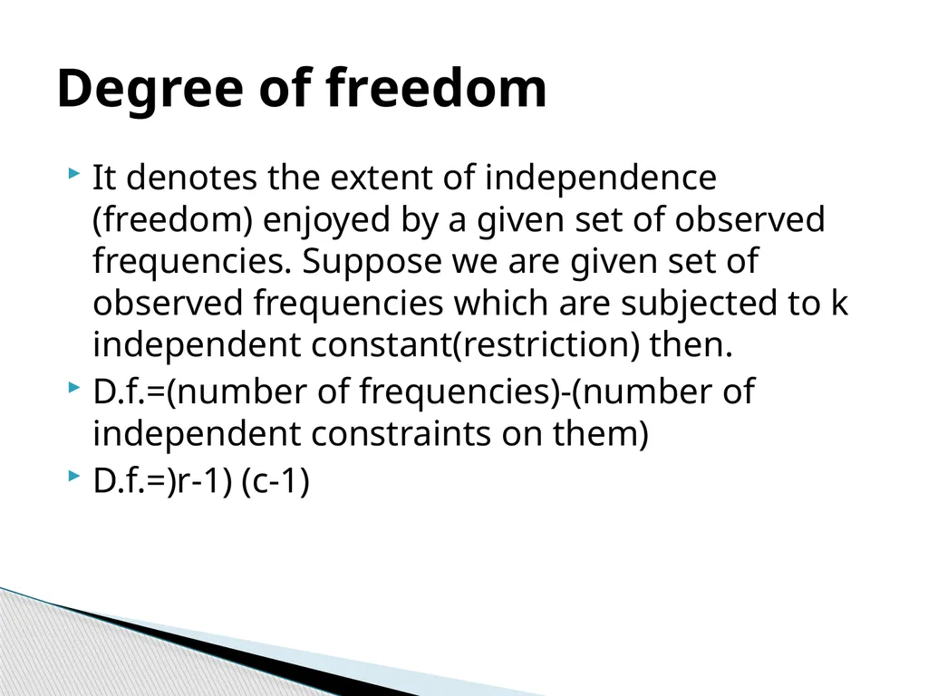
It denotes the extent of independence (freedom) enjoyed by a given set of observed frequencies. Suppose we are given set of observed frequencies which are subjected to k independent constant(restriction) then.
D.f.=(number of frequencies)-(number of independent constraints on them)
D.f.=)r-1) (c-1) Degree of freedom<br>
D.f.=(number of frequencies)-(number of independent constraints on them)
D.f.=)r-1) (c-1) Degree of freedom<br>
07
1 or more categories
Independent observations
A sample size of at least 10
Random sampling
All observations must be used
For the test to be accurate, the expected frequency should be at least 5 Assumptions of Chi-square<br>
Independent observations
A sample size of at least 10
Random sampling
All observations must be used
For the test to be accurate, the expected frequency should be at least 5 Assumptions of Chi-square<br>
08
Implying cause rather than association
Overestimating the importance of a finding, especially with large sample sizes
Failure to recognize spurious relationships
Nominal variables only (both IV and DV) Chi-Square Limits & Problems<br>
Overestimating the importance of a finding, especially with large sample sizes
Failure to recognize spurious relationships
Nominal variables only (both IV and DV) Chi-Square Limits & Problems<br>
09
A chi-square analysis is not used to prove a hypothesis; it can, however, refute one.
As the chi-square value increases, the probability that the experimental outcome could occur by random chance decreases.
The results of a chi-square analysis tell you: Whether the difference between what you observe and the level of difference is due to sampling error.
The greater the deviation of what we observe to what we would expect by chance, the greater the probability that the difference is NOT due to chance. Chi-Square Attributes<br>
As the chi-square value increases, the probability that the experimental outcome could occur by random chance decreases.
The results of a chi-square analysis tell you: Whether the difference between what you observe and the level of difference is due to sampling error.
The greater the deviation of what we observe to what we would expect by chance, the greater the probability that the difference is NOT due to chance. Chi-Square Attributes<br>
10
Critical values for chi-square are found on tables, sorted by degrees of freedom and probability levels. Be sure to use p < 0.05.
If your calculated chi-square value is greater than the critical value calculated, you“reject the null hypothesis.”
If your chi-square value is less than the critical value, you“fail to reject” the null hypothesis Critical Chi-Square Values<br>
If your calculated chi-square value is greater than the critical value calculated, you“reject the null hypothesis.”
If your chi-square value is less than the critical value, you“fail to reject” the null hypothesis Critical Chi-Square Values<br>
11
To test the null hypothesis, compare the frequencies which were observed with the frequencies we expect to observe if the null hypothesis is true
If the differences between the observed and the expected are small, that supports the null hypothesis
If the differences between the observed and the expected are large, we will be inclined to reject the null hypothesis Hypothesis Testing with X2<br>
If the differences between the observed and the expected are small, that supports the null hypothesis
If the differences between the observed and the expected are large, we will be inclined to reject the null hypothesis Hypothesis Testing with X2<br>
12
Normally requires sufficiently large sample size:
In general N > 20.
No one accepted cutoff – the general rules are
No cells with observed frequency = 0
No cells with the expected frequency < 5
Applying chi-square to very small samples exposes the researcher to an unacceptable rate of Type II errors.
Note: chi-square must be calculated on actual count data, not substituting percentages, which would have the effect of pretending the sample size is 100. Chi-Square Use Assumptions<br>
In general N > 20.
No one accepted cutoff – the general rules are
No cells with observed frequency = 0
No cells with the expected frequency < 5
Applying chi-square to very small samples exposes the researcher to an unacceptable rate of Type II errors.
Note: chi-square must be calculated on actual count data, not substituting percentages, which would have the effect of pretending the sample size is 100. Chi-Square Use Assumptions<br>
13
Conceptually, the chi-square test of independence statistic is computed by summing the difference between the expected and observed frequencies for each cell in the table divided by the expected frequencies for the cell.
We identify the value and probability for this test statistic from the SPSS statistical output.
If the probability of the test statistic is less than or equal to the probability of the alpha error rate, we reject the null hypothesis and conclude that our data supports the research hypothesis. We conclude that there is a relationship between the variables.
If the probability of the test statistic is greater than the probability of the alpha error rate, we fail to reject the null hypothesis. We conclude that there is no relationship between the variables, i.e. they are independent. Using SPSS for Calculating X2<br>
We identify the value and probability for this test statistic from the SPSS statistical output.
If the probability of the test statistic is less than or equal to the probability of the alpha error rate, we reject the null hypothesis and conclude that our data supports the research hypothesis. We conclude that there is a relationship between the variables.
If the probability of the test statistic is greater than the probability of the alpha error rate, we fail to reject the null hypothesis. We conclude that there is no relationship between the variables, i.e. they are independent. Using SPSS for Calculating X2<br>
14
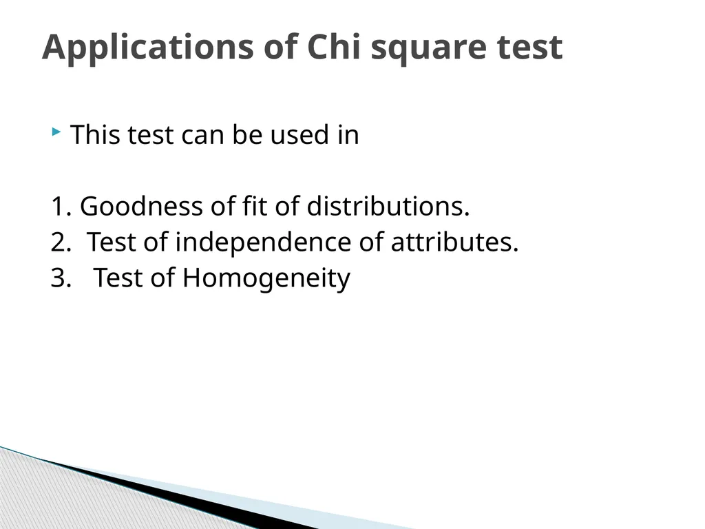
This test can be used in
1. Goodness of fit of distributions.
2. Test of independence of attributes.
3. Test of Homogeneity Applications of Chi square test<br>
1. Goodness of fit of distributions.
2. Test of independence of attributes.
3. Test of Homogeneity Applications of Chi square test<br>
15
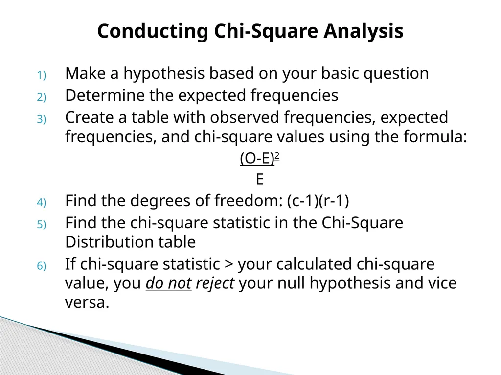
Make a hypothesis based on your basic question
Determine the expected frequencies
Create a table with observed frequencies, expected frequencies, and chi-square values using the formula:
(O-E)2
E
Find the degrees of freedom: (c-1)(r-1)
Find the chi-square statistic in the Chi-Square Distribution table
If chi-square statistic > your calculated chi-square value, you do not reject your null hypothesis and vice versa. Conducting Chi-Square Analysis<br>
Determine the expected frequencies
Create a table with observed frequencies, expected frequencies, and chi-square values using the formula:
(O-E)2
E
Find the degrees of freedom: (c-1)(r-1)
Find the chi-square statistic in the Chi-Square Distribution table
If chi-square statistic > your calculated chi-square value, you do not reject your null hypothesis and vice versa. Conducting Chi-Square Analysis<br>
16
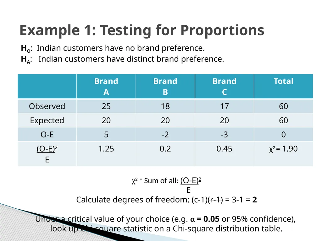
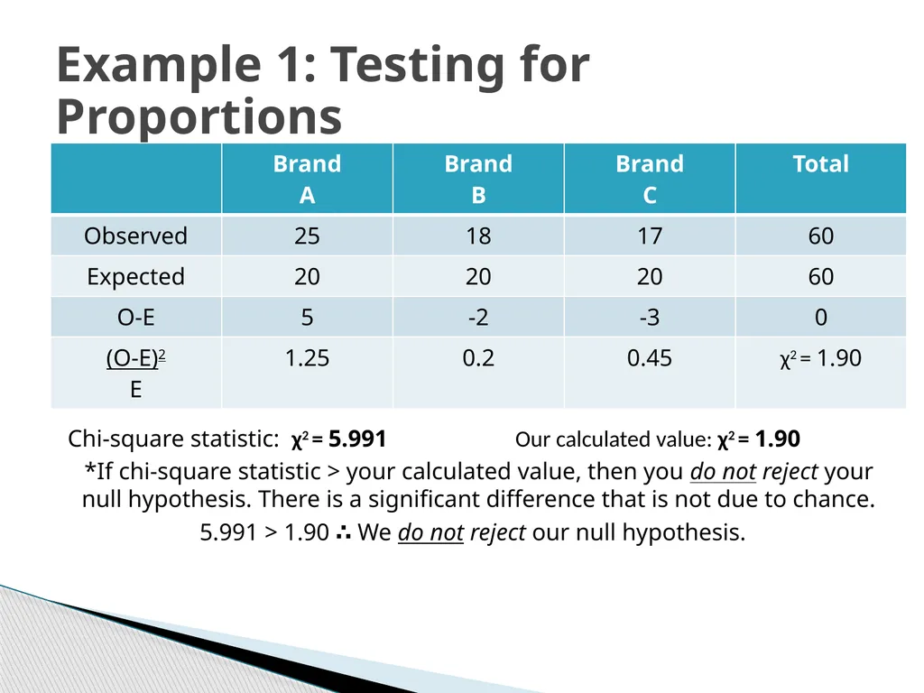
Example 1: Testing for Proportions HO: Indian customers have no brand preference.
HA: Indian customers have distinct brand preference. χ2 = Sum of all: (O-E)2
E
Calculate degrees of freedom: (c-1)(r-1) = 3-1 = 2
Under a critical value of your choice (e.g. α = 0.05 or 95% confidence),
look up Chi-square statistic on a Chi-square distribution table.<br>
HA: Indian customers have distinct brand preference. χ2 = Sum of all: (O-E)2
E
Calculate degrees of freedom: (c-1)(r-1) = 3-1 = 2
Under a critical value of your choice (e.g. α = 0.05 or 95% confidence),
look up Chi-square statistic on a Chi-square distribution table.<br>
17
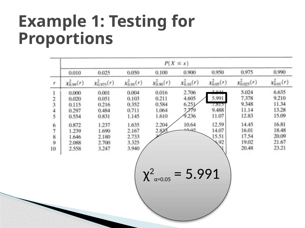
Example 1: Testing for Proportions χ2α=0.05 = 5.991<br>
18
Chi-square statistic: χ2 = 5.991 Our calculated value: χ2 = 1.90
*If chi-square statistic > your calculated value, then you do not reject your null hypothesis. There is a significant difference that is not due to chance.
5.991 > 1.90 ∴ We do not reject our null hypothesis. Example 1: Testing for Proportions<br>
*If chi-square statistic > your calculated value, then you do not reject your null hypothesis. There is a significant difference that is not due to chance.
5.991 > 1.90 ∴ We do not reject our null hypothesis. Example 1: Testing for Proportions<br>
19
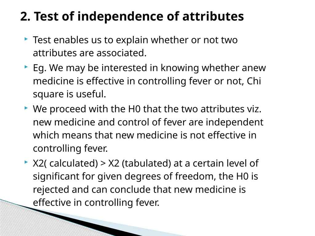
Test enables us to explain whether or not two attributes are associated.
Eg. We may be interested in knowing whether anew medicine is effective in controlling fever or not, Chi square is useful.
We proceed with the H0 that the two attributes viz. new medicine and control of fever are independent which means that new medicine is not effective in controlling fever.
X2( calculated) > X2 (tabulated) at a certain level of significant for given degrees of freedom, the H0 is rejected and can conclude that new medicine is effective in controlling fever. 2. Test of independence of attributes<br>
Eg. We may be interested in knowing whether anew medicine is effective in controlling fever or not, Chi square is useful.
We proceed with the H0 that the two attributes viz. new medicine and control of fever are independent which means that new medicine is not effective in controlling fever.
X2( calculated) > X2 (tabulated) at a certain level of significant for given degrees of freedom, the H0 is rejected and can conclude that new medicine is effective in controlling fever. 2. Test of independence of attributes<br>
20
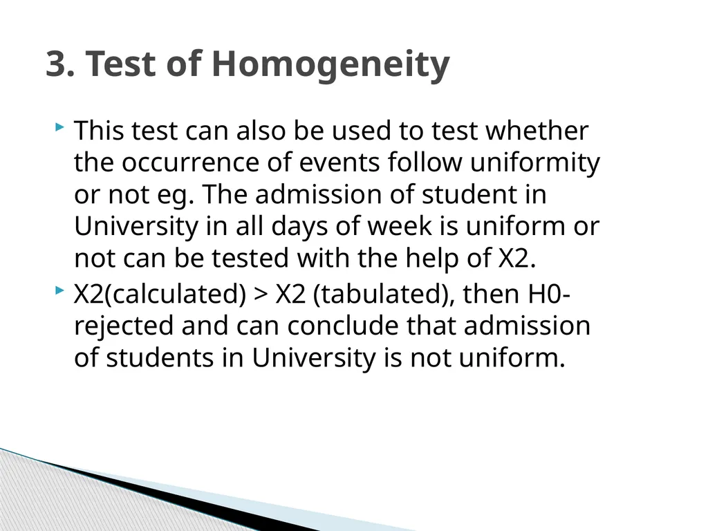
This test can also be used to test whether the occurrence of events follow uniformity or not eg. The admission of student in University in all days of week is uniform or not can be tested with the help of X2.
X2(calculated) > X2 (tabulated), then H0- rejected and can conclude that admission of students in University is not uniform. 3. Test of Homogeneity<br>
X2(calculated) > X2 (tabulated), then H0- rejected and can conclude that admission of students in University is not uniform. 3. Test of Homogeneity<br>
21
Eg.2 Suppose we want to toss 50 times a coin<br>
22
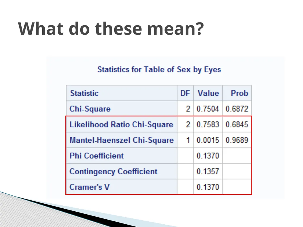
What do these mean?<br>
23
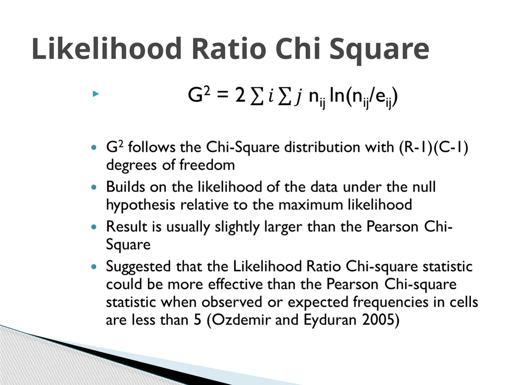
Likelihood Ratio Chi Square<br>
24
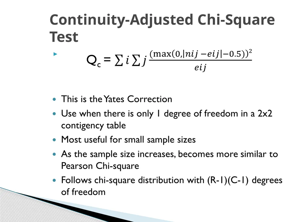
Continuity-Adjusted Chi-Square Test<br>
25
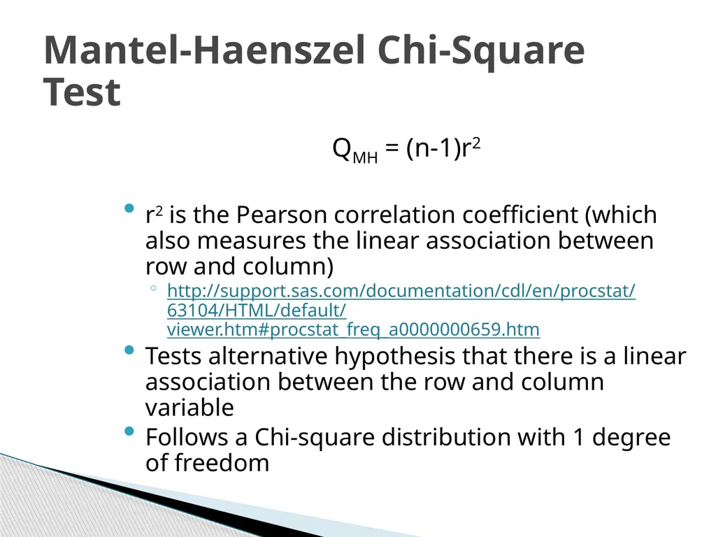
QMH = (n-1)r2
r2 is the Pearson correlation coefficient (which also measures the linear association between row and column)
http://support.sas.com/documentation/cdl/en/procstat/63104/HTML/default/viewer.htm#procstat_freq_a0000000659.htm
Tests alternative hypothesis that there is a linear association between the row and column variable
Follows a Chi-square distribution with 1 degree of freedom Mantel-Haenszel Chi-Square Test<br>
r2 is the Pearson correlation coefficient (which also measures the linear association between row and column)
http://support.sas.com/documentation/cdl/en/procstat/63104/HTML/default/viewer.htm#procstat_freq_a0000000659.htm
Tests alternative hypothesis that there is a linear association between the row and column variable
Follows a Chi-square distribution with 1 degree of freedom Mantel-Haenszel Chi-Square Test<br>
26
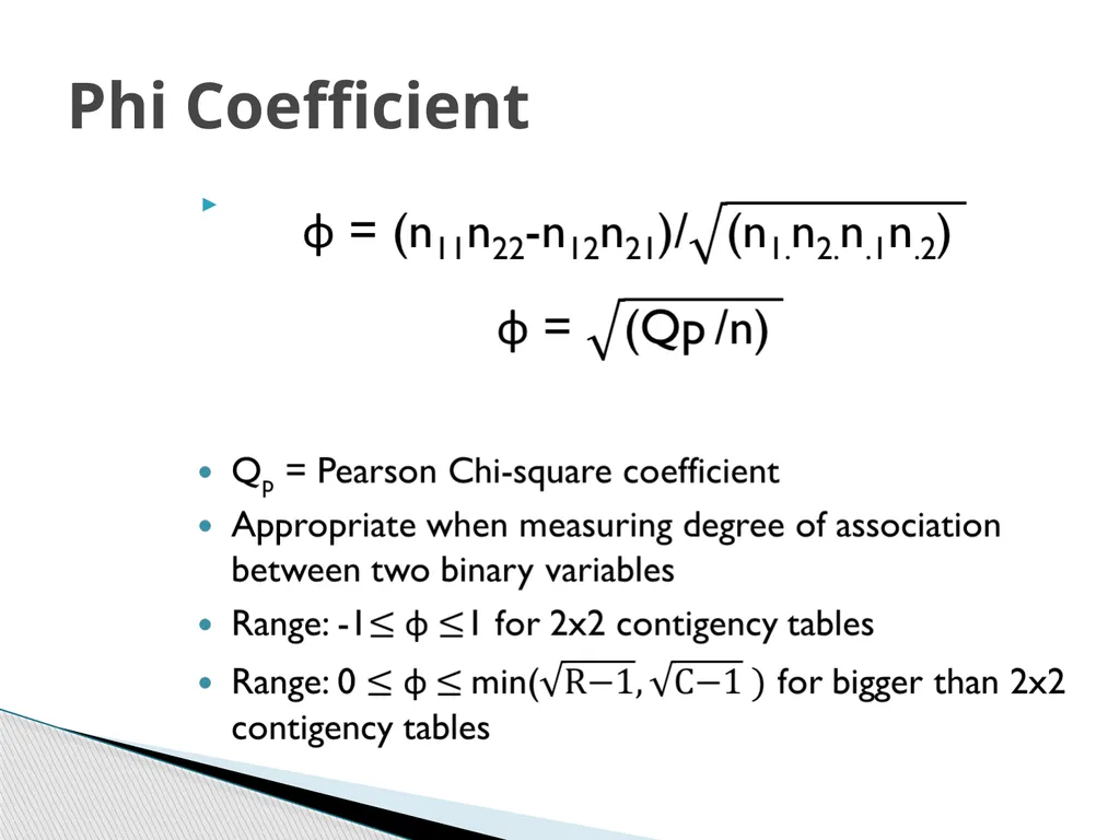
Phi Coefficient<br>
27
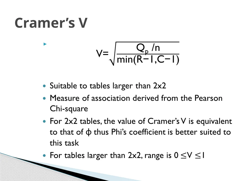
Cramer’s V<br>
28
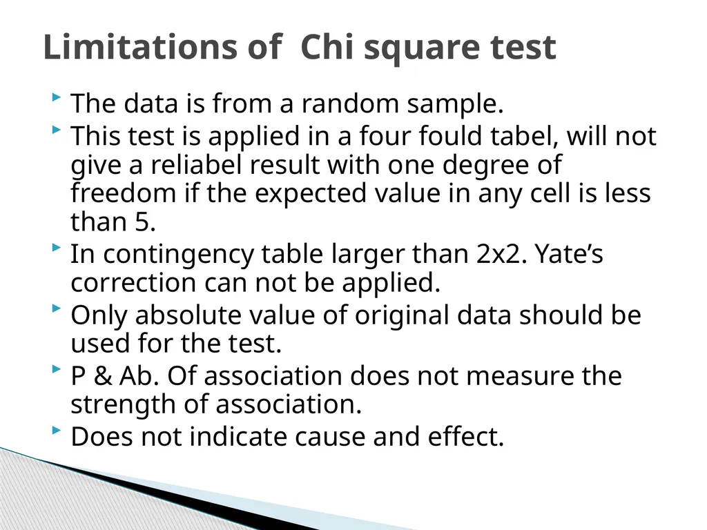
The data is from a random sample.
This test is applied in a four fould tabel, will not give a reliabel result with one degree of freedom if the expected value in any cell is less than 5.
In contingency table larger than 2x2. Yate’s correction can not be applied.
Only absolute value of original data should be used for the test.
P & Ab. Of association does not measure the strength of association.
Does not indicate cause and effect. Limitations of Chi square test<br>
This test is applied in a four fould tabel, will not give a reliabel result with one degree of freedom if the expected value in any cell is less than 5.
In contingency table larger than 2x2. Yate’s correction can not be applied.
Only absolute value of original data should be used for the test.
P & Ab. Of association does not measure the strength of association.
Does not indicate cause and effect. Limitations of Chi square test<br>