
Class 5 Option Contracts Options A call option is
KL
Published · 52 slides · 0 views
1 / 1

Description
Class 5 Option Contracts Options A call option is a contract that gives the buyer the right, but not the obligation, to buy the underlying security at a prespecified price (called the strike or exercise price) within a prespecified period
Related Topics
Share
Embed code
Download this presentation From Below
"Class 5 Option Contracts Options A call option is" is the property of its rightful owner. Permission is granted to download and print the materials on this website for personal, non-commercial use only, and to display it on your personal computer provided you do not modify the materials and that you retain all copyright notices contained in the materials. By downloading content from our website, you accept the terms of this agreement.
Presentation Transcript
01
Class 5 Option Contracts<br>
02
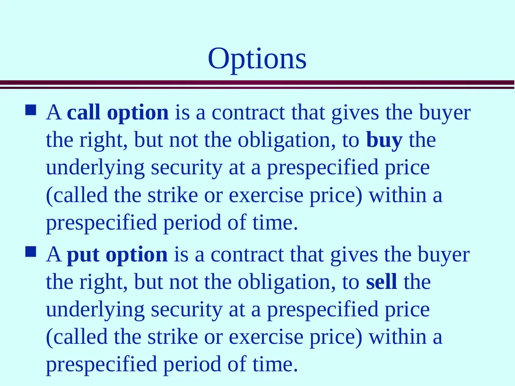
Options A call option is a contract that gives the buyer the right, but not the obligation, to buy the underlying security at a prespecified price (called the strike or exercise price) within a prespecified period of time.
A put option is a contract that gives the buyer the right, but not the obligation, to sell the underlying security at a prespecified price (called the strike or exercise price) within a prespecified period of time.<br>
A put option is a contract that gives the buyer the right, but not the obligation, to sell the underlying security at a prespecified price (called the strike or exercise price) within a prespecified period of time.<br>
03
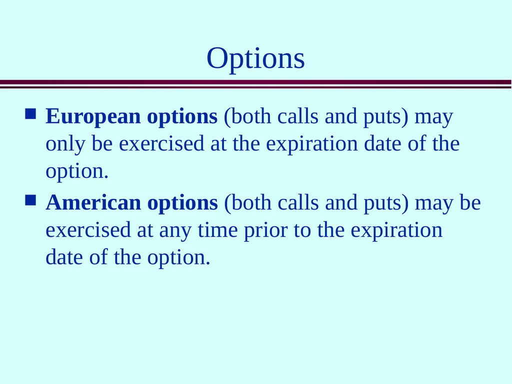
Options European options (both calls and puts) may only be exercised at the expiration date of the option.
American options (both calls and puts) may be exercised at any time prior to the expiration date of the option.<br>
American options (both calls and puts) may be exercised at any time prior to the expiration date of the option.<br>
04
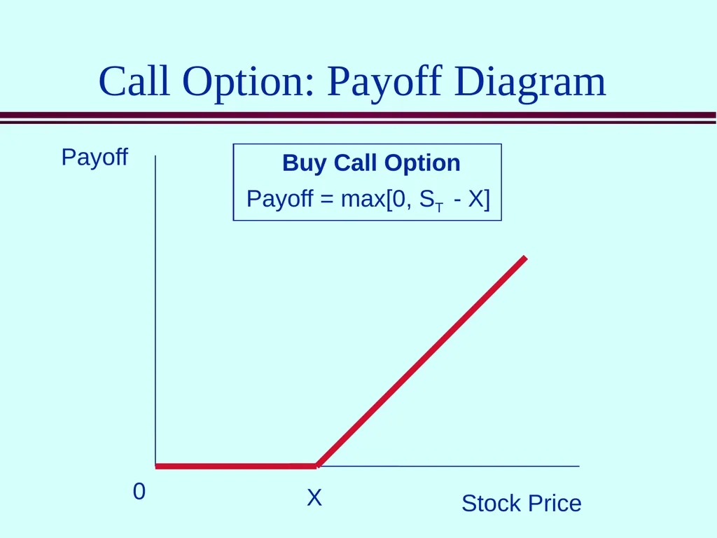
Call Option: Payoff Diagram Payoff Stock Price X 0 Payoff = max[0, ST - X] Buy Call Option<br>
05
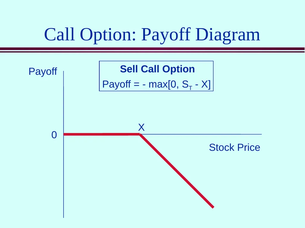
Call Option: Payoff Diagram Payoff Stock Price X 0 Sell Call Option Payoff = - max[0, ST - X]<br>
06
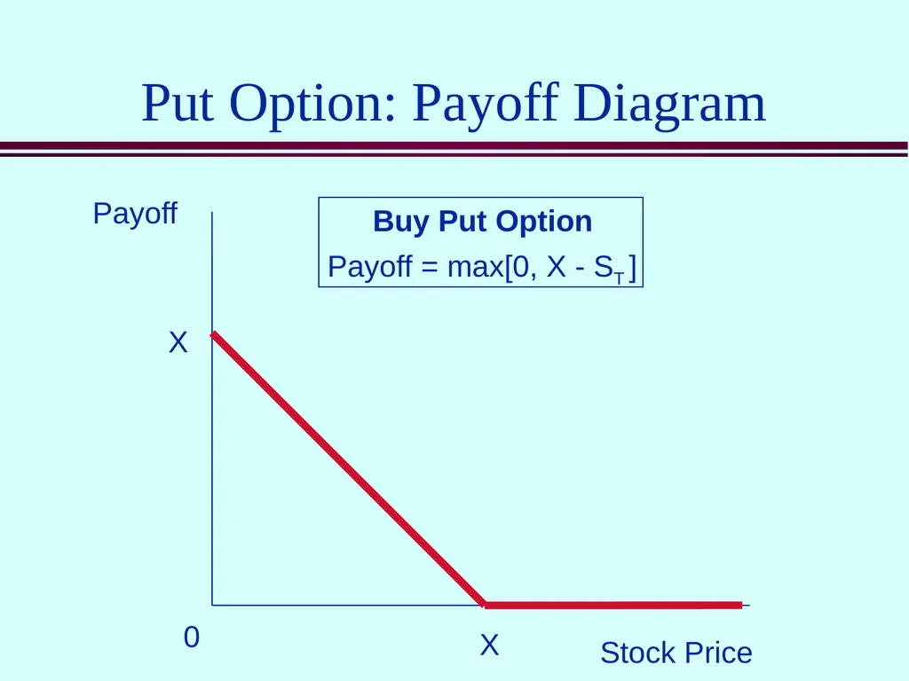
Put Option: Payoff Diagram Payoff Stock Price X 0 Payoff = max[0, X - ST ] Buy Put Option X<br>
07
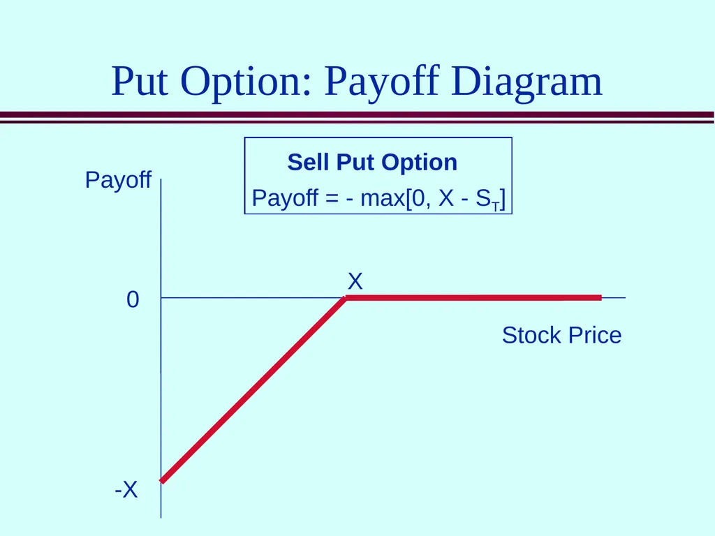
Put Option: Payoff Diagram Payoff Stock Price X 0 Sell Put Option Payoff = - max[0, X - ST] -X<br>
08
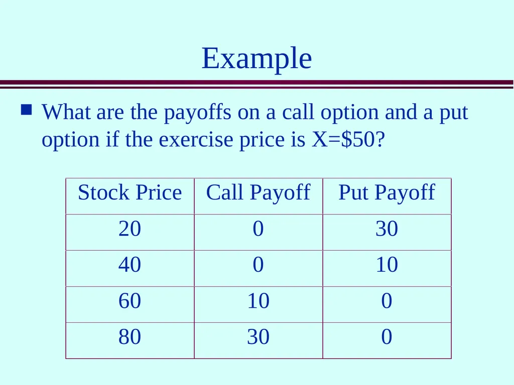
Example What are the payoffs on a call option and a put option if the exercise price is X=$50?<br>
09
Option Trading Strategies:
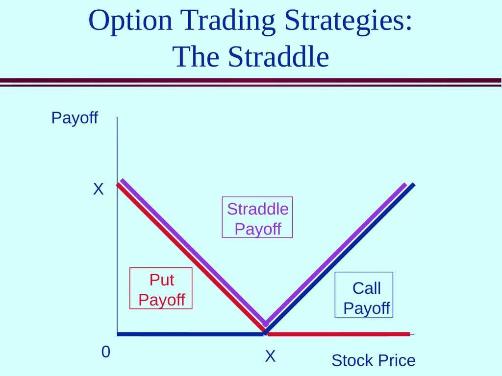
The Straddle Buy a call and a put on the same stock with the same exercise price and time to maturity.
Appropriate when you believe the stock price will change a lot, but you are unsure of the direction.<br>
Appropriate when you believe the stock price will change a lot, but you are unsure of the direction.<br>
10
Option Trading Strategies:
The Straddle Payoff Stock Price X 0 X Put
Payoff Call
Payoff Straddle
Payoff<br>
Payoff Call
Payoff Straddle
Payoff<br>
11
Option Trading Strategies:
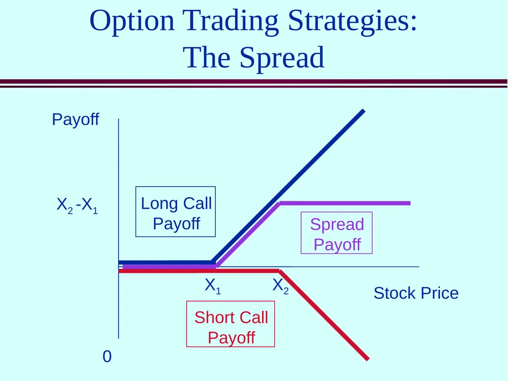
The Spread Buy a call and sell another call with a higher strike price on the same stock with the same time to maturity.
Appropriate when you believe the stock price will increase and you are willing to trade off some upside potential to reduce the cost of your investment.<br>
Appropriate when you believe the stock price will increase and you are willing to trade off some upside potential to reduce the cost of your investment.<br>
12
Option Trading Strategies:
The Spread Payoff Stock Price X1 0 Short Call
Payoff Long Call
Payoff Spread
Payoff X2 X2 -X1<br>
Payoff Long Call
Payoff Spread
Payoff X2 X2 -X1<br>
13
Valuation of Options:
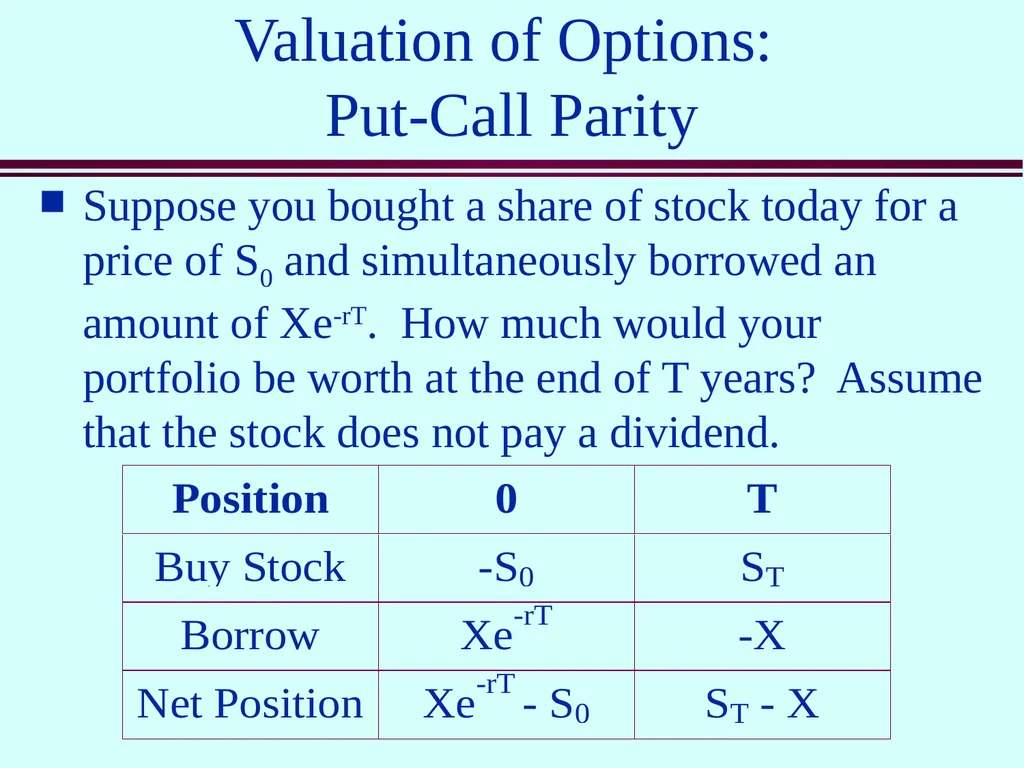
Put-Call Parity Suppose you bought a share of stock today for a price of S0 and simultaneously borrowed an amount of Xe-rT. How much would your portfolio be worth at the end of T years? Assume that the stock does not pay a dividend.<br>
14
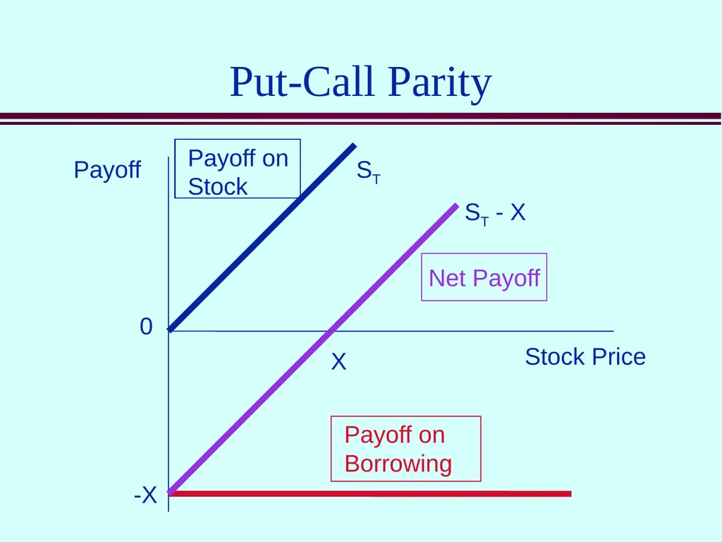
Put-Call Parity Payoff Stock Price ST -X ST - X 0 Payoff on Stock Payoff on Borrowing Net Payoff X<br>
15
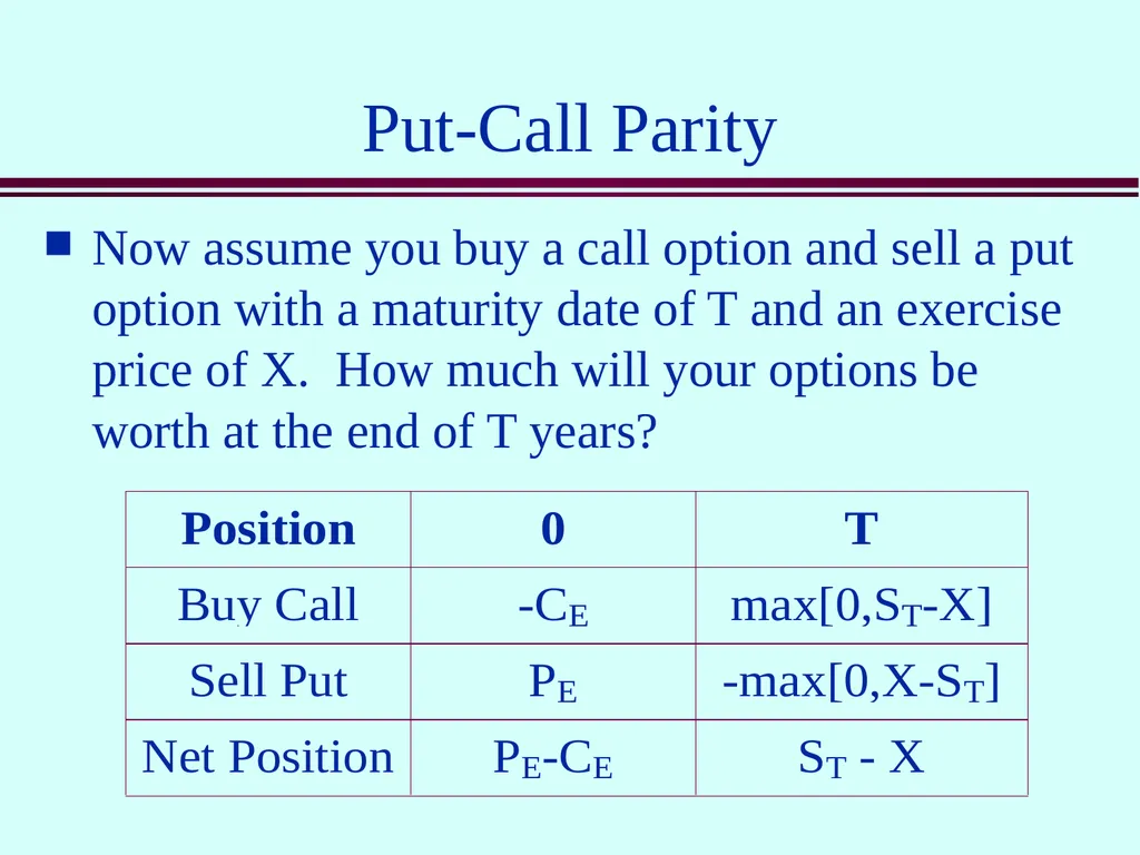
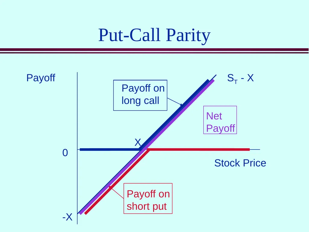
Put-Call Parity Now assume you buy a call option and sell a put option with a maturity date of T and an exercise price of X. How much will your options be worth at the end of T years?<br>
16
Put-Call Parity Payoff Stock Price -X X ST - X 0 Payoff on short put Payoff on long call Net
Payoff<br>
Payoff<br>
17
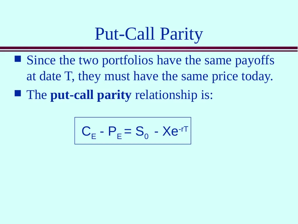
Put-Call Parity Since the two portfolios have the same payoffs at date T, they must have the same price today.
The put-call parity relationship is: CE - PE = S0 - Xe-rT<br>
The put-call parity relationship is: CE - PE = S0 - Xe-rT<br>
18
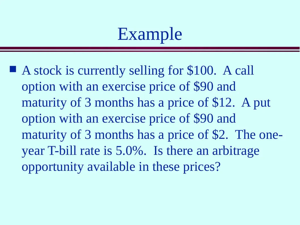
Example A stock is currently selling for $100. A call option with an exercise price of $90 and maturity of 3 months has a price of $12. A put option with an exercise price of $90 and maturity of 3 months has a price of $2. The one-year T-bill rate is 5.0%. Is there an arbitrage opportunity available in these prices?<br>
19
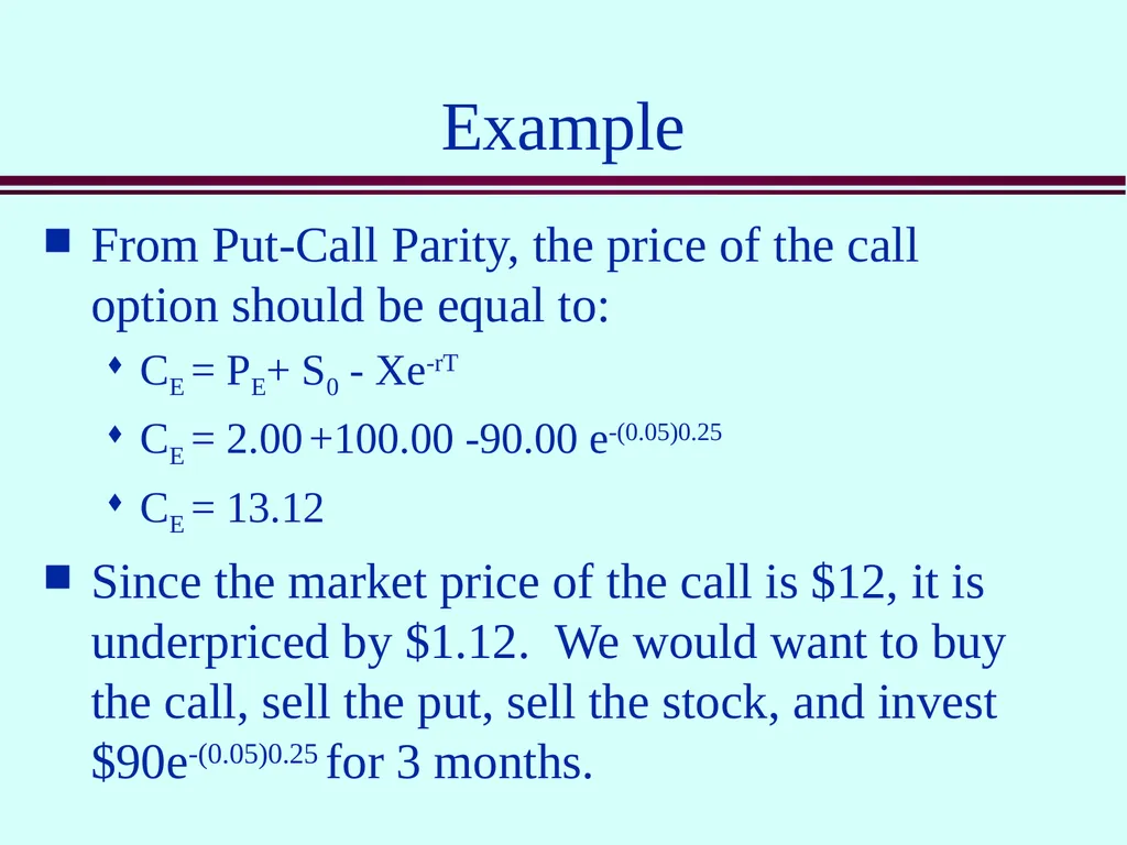
Example From Put-Call Parity, the price of the call option should be equal to:
CE = PE+ S0 - Xe-rT
CE = 2.00 +100.00 -90.00 e-(0.05)0.25
CE = 13.12
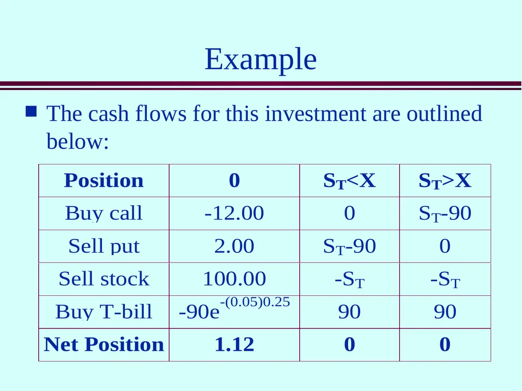
Since the market price of the call is $12, it is underpriced by $1.12. We would want to buy the call, sell the put, sell the stock, and invest $90e-(0.05)0.25 for 3 months.<br>
CE = PE+ S0 - Xe-rT
CE = 2.00 +100.00 -90.00 e-(0.05)0.25
CE = 13.12
Since the market price of the call is $12, it is underpriced by $1.12. We would want to buy the call, sell the put, sell the stock, and invest $90e-(0.05)0.25 for 3 months.<br>
20
Example The cash flows for this investment are outlined below:<br>
21
Lower Bounds for
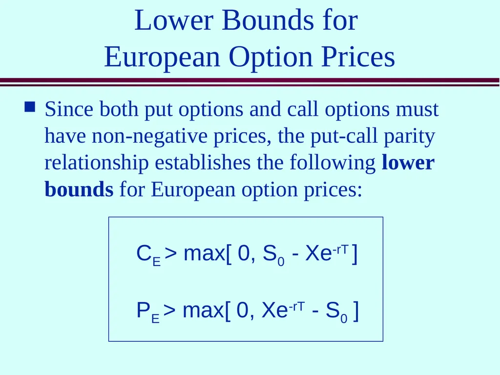
European Option Prices Since both put options and call options must have non-negative prices, the put-call parity relationship establishes the following lower bounds for European option prices: CE > max[ 0, S0 - Xe-rT ]
PE > max[ 0, Xe-rT - S0 ]<br>
PE > max[ 0, Xe-rT - S0 ]<br>
22
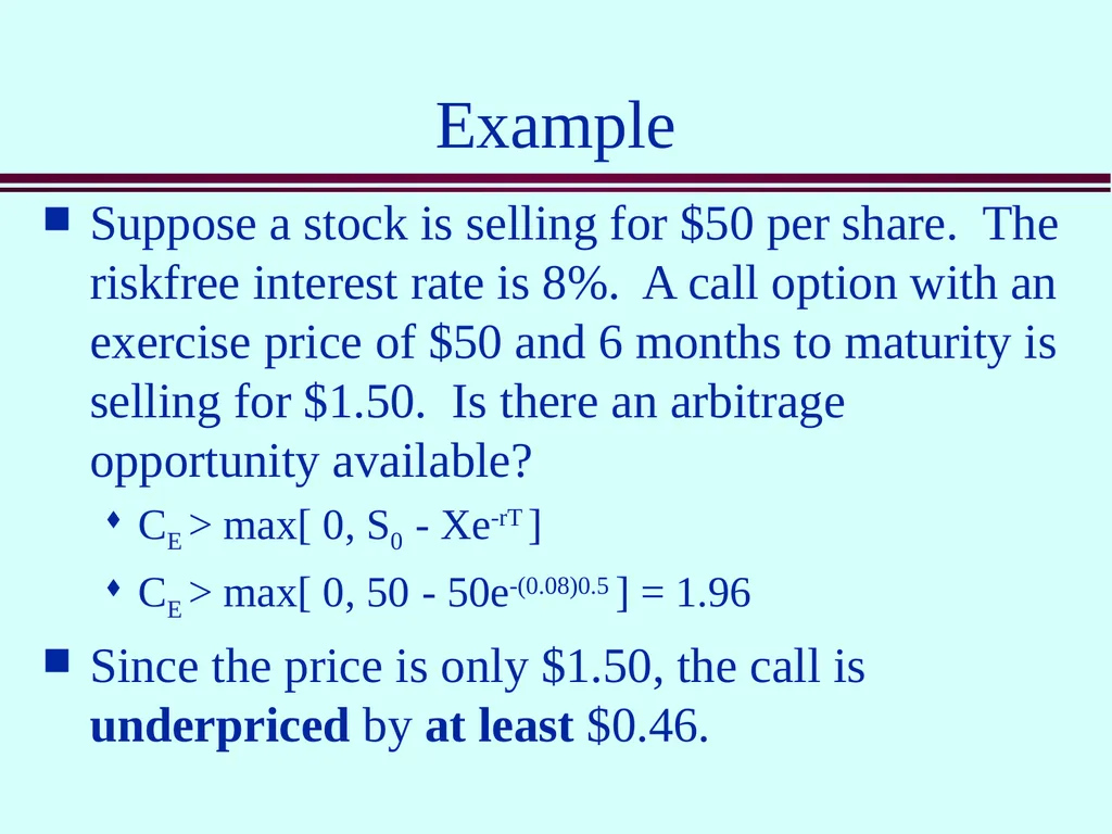
Example Suppose a stock is selling for $50 per share. The riskfree interest rate is 8%. A call option with an exercise price of $50 and 6 months to maturity is selling for $1.50. Is there an arbitrage opportunity available?
CE > max[ 0, S0 - Xe-rT ]
CE > max[ 0, 50 - 50e-(0.08)0.5 ] = 1.96
Since the price is only $1.50, the call is underpriced by at least $0.46.<br>
CE > max[ 0, S0 - Xe-rT ]
CE > max[ 0, 50 - 50e-(0.08)0.5 ] = 1.96
Since the price is only $1.50, the call is underpriced by at least $0.46.<br>
23
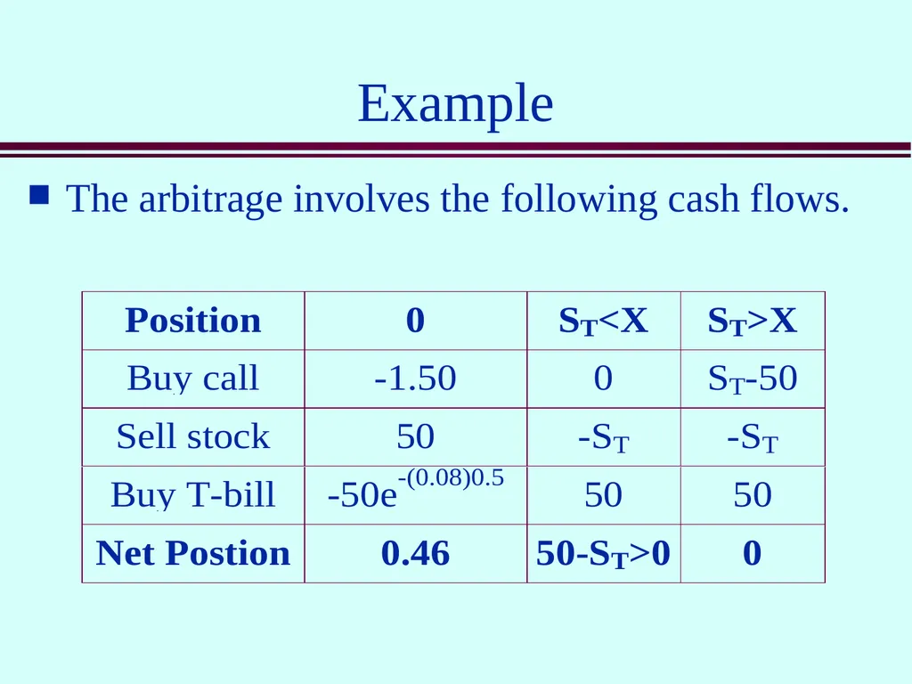
Example The arbitrage involves the following cash flows.<br>
24
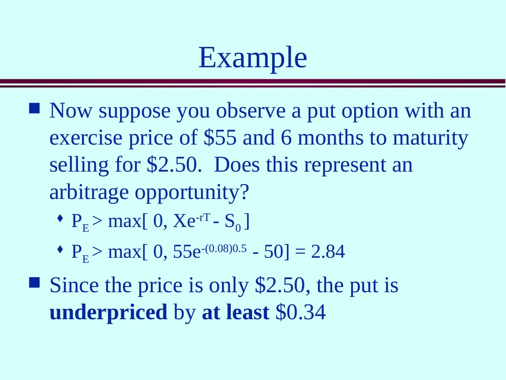
Example Now suppose you observe a put option with an exercise price of $55 and 6 months to maturity selling for $2.50. Does this represent an arbitrage opportunity?
PE > max[ 0, Xe-rT - S0 ]
PE > max[ 0, 55e-(0.08)0.5 - 50] = 2.84
Since the price is only $2.50, the put is underpriced by at least $0.34<br>
PE > max[ 0, Xe-rT - S0 ]
PE > max[ 0, 55e-(0.08)0.5 - 50] = 2.84
Since the price is only $2.50, the put is underpriced by at least $0.34<br>
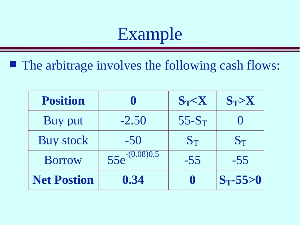
25
Example The arbitrage involves the following cash flows:<br>
26
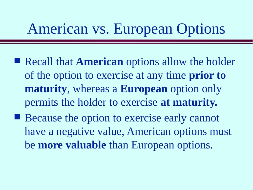
American vs. European Options Recall that American options allow the holder of the option to exercise at any time prior to maturity, whereas a European option only permits the holder to exercise at maturity.
Because the option to exercise early cannot have a negative value, American options must be more valuable than European options.<br>
Because the option to exercise early cannot have a negative value, American options must be more valuable than European options.<br>
27
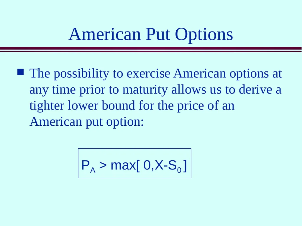
American Put Options The possibility to exercise American options at any time prior to maturity allows us to derive a tighter lower bound for the price of an American put option: PA > max[ 0,X-S0 ]<br>
28
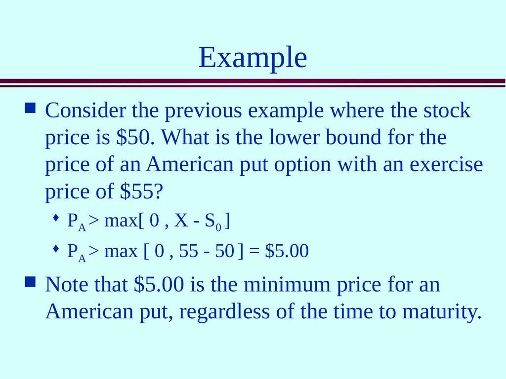
Example Consider the previous example where the stock price is $50. What is the lower bound for the price of an American put option with an exercise price of $55?
PA > max[ 0 , X - S0 ]
PA > max [ 0 , 55 - 50 ] = $5.00
Note that $5.00 is the minimum price for an American put, regardless of the time to maturity.<br>
PA > max[ 0 , X - S0 ]
PA > max [ 0 , 55 - 50 ] = $5.00
Note that $5.00 is the minimum price for an American put, regardless of the time to maturity.<br>
29
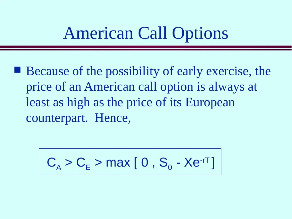
American Call Options Because of the possibility of early exercise, the price of an American call option is always at least as high as the price of its European counterpart. Hence, CA > CE > max [ 0 , S0 - Xe-rT ]<br>
30
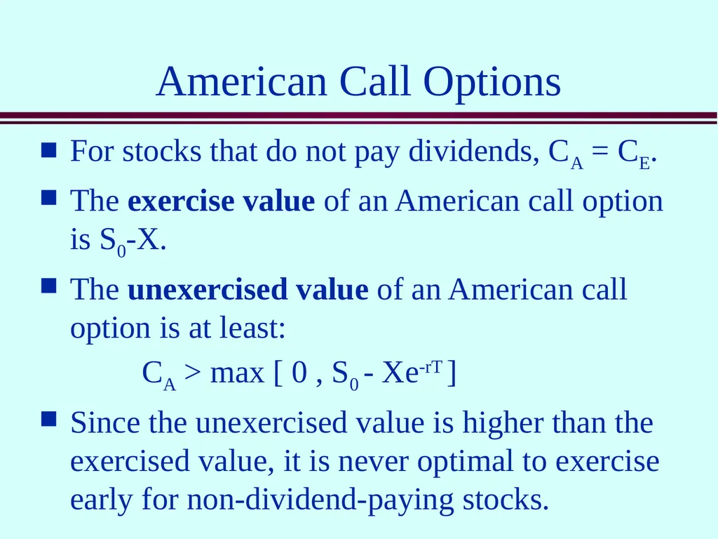
American Call Options For stocks that do not pay dividends, CA = CE.
The exercise value of an American call option is S0-X.
The unexercised value of an American call option is at least:
CA > max [ 0 , S0 - Xe-rT ]
Since the unexercised value is higher than the exercised value, it is never optimal to exercise early for non-dividend-paying stocks.<br>
The exercise value of an American call option is S0-X.
The unexercised value of an American call option is at least:
CA > max [ 0 , S0 - Xe-rT ]
Since the unexercised value is higher than the exercised value, it is never optimal to exercise early for non-dividend-paying stocks.<br>
31
Black-Scholes Option
Pricing Formula The Black-Scholes option pricing formula prices European options on non-dividend-paying stocks.
Black-Scholes Call Option Formula:
N(d1) = cumulative normal probability distribution, or NORMSDIST(.) in EXCEL. CE = S N(d1) - Xe-rT N(d2)<br>
Black-Scholes Call Option Formula:
N(d1) = cumulative normal probability distribution, or NORMSDIST(.) in EXCEL. CE = S N(d1) - Xe-rT N(d2)<br>
32
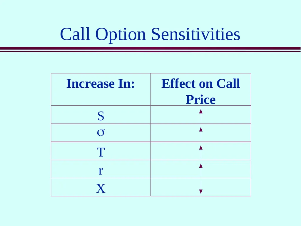
Call Option Sensitivities<br>
33
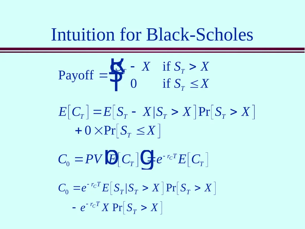
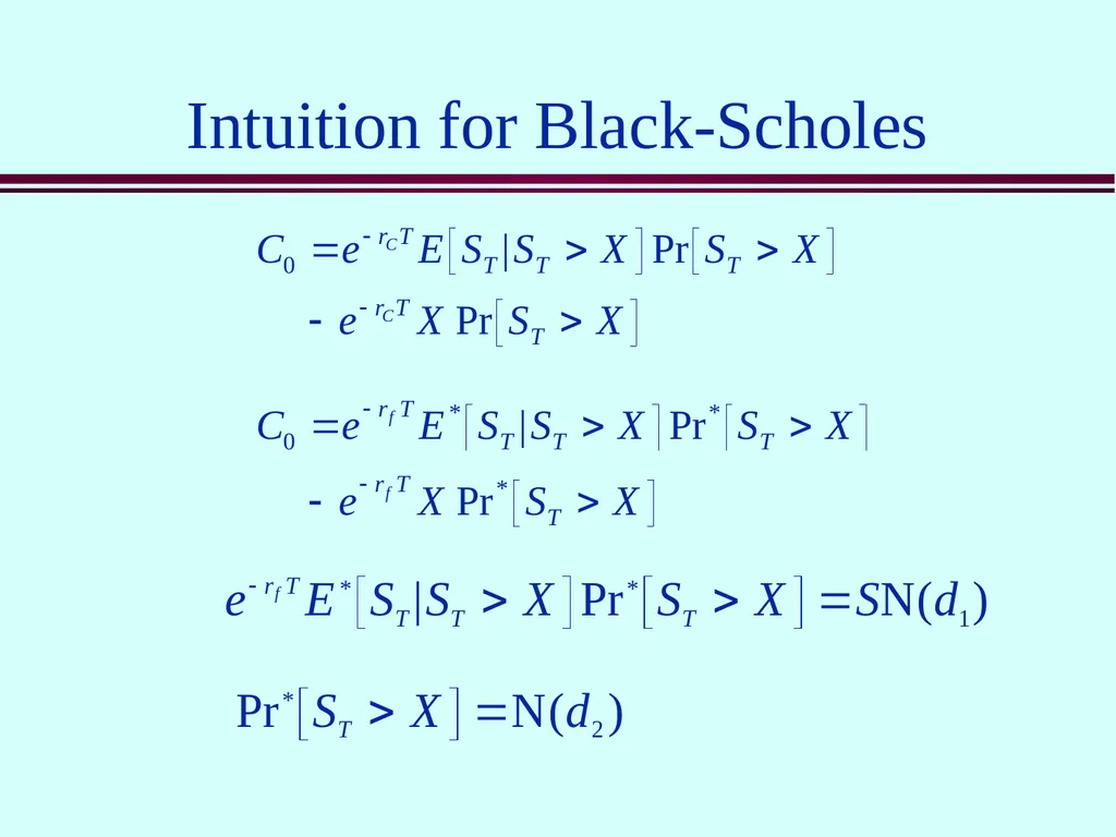
Intuition for Black-Scholes<br>
34
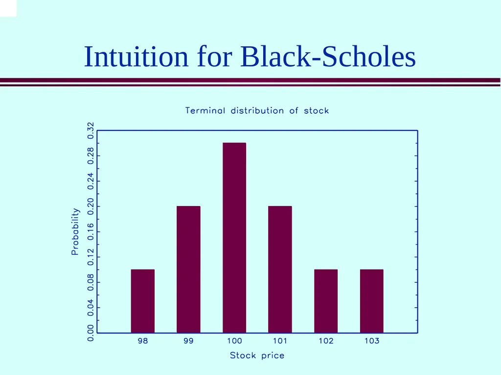
Intuition for Black-Scholes<br>
35
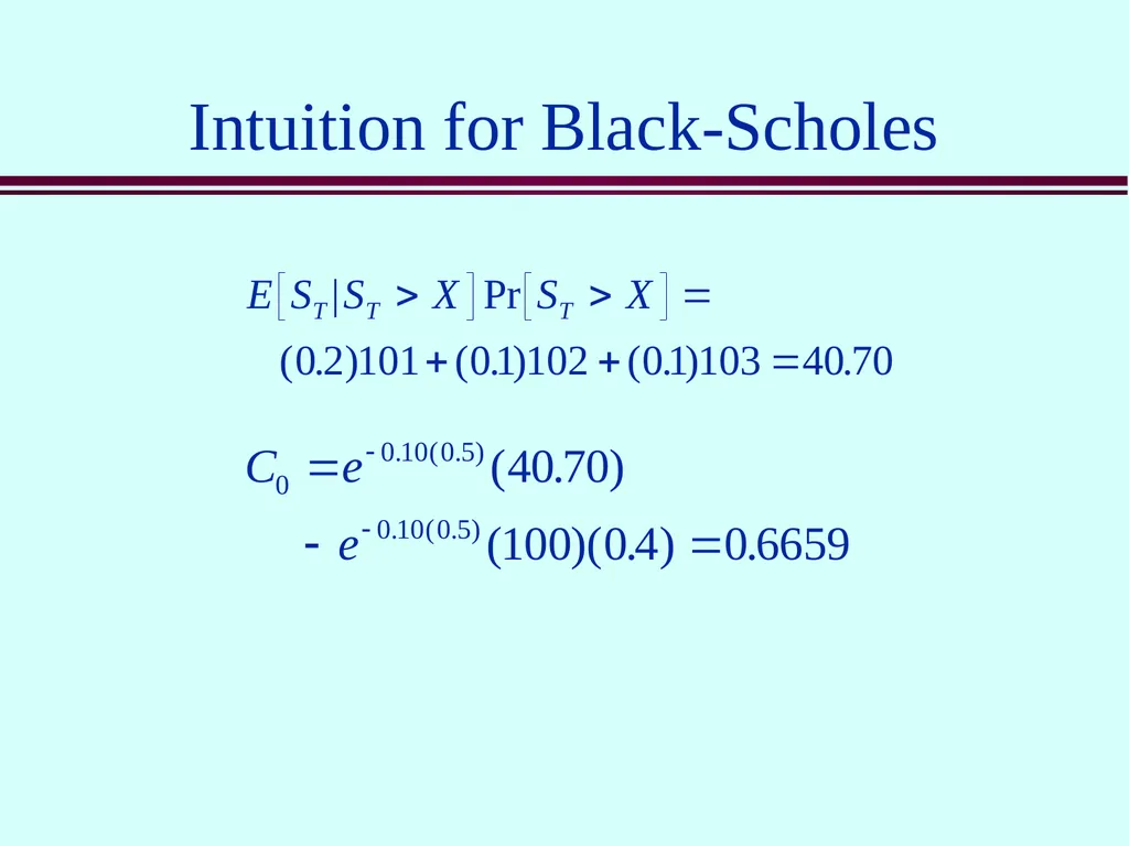
Intuition for Black-Scholes<br>
36
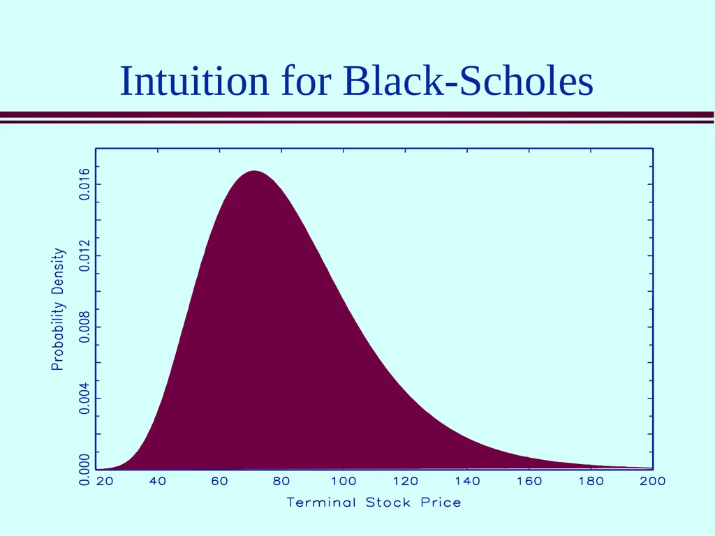
Intuition for Black-Scholes<br>
37
Intuition for Black-Scholes<br>
38
Black-Scholes Put
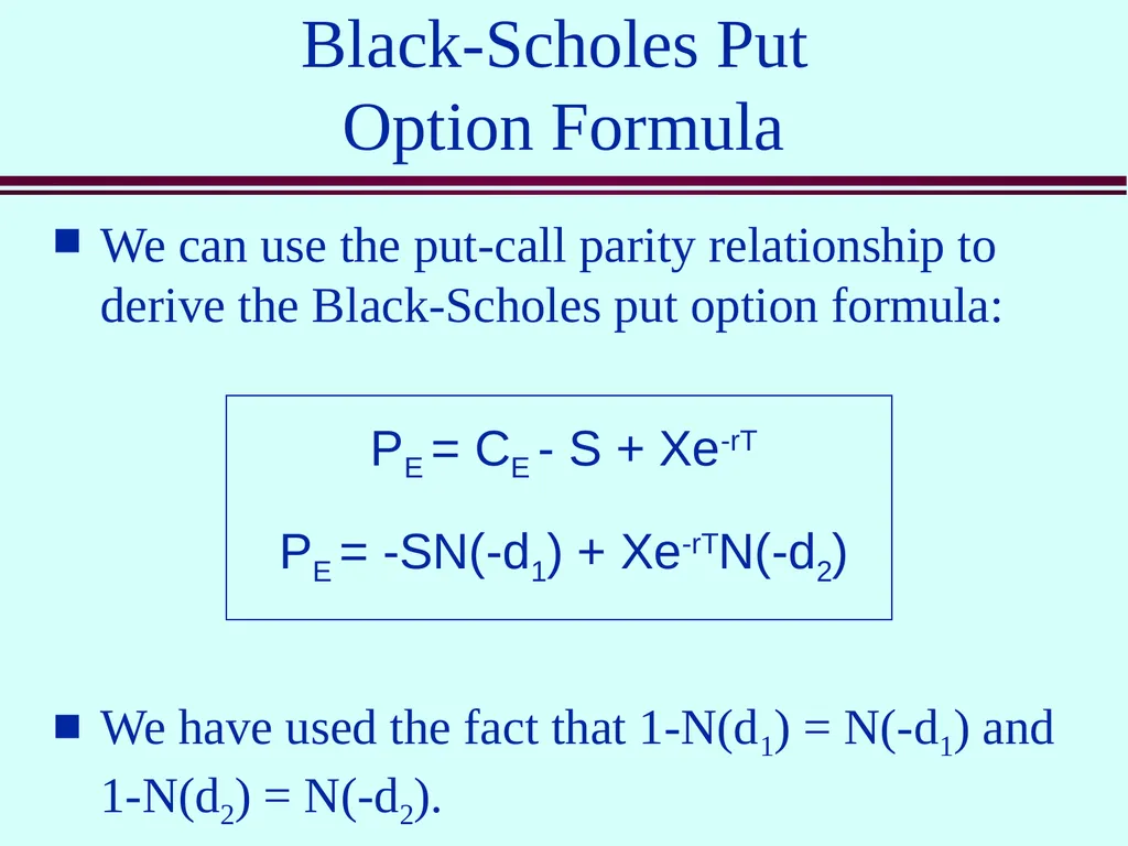
Option Formula We can use the put-call parity relationship to derive the Black-Scholes put option formula:
We have used the fact that 1-N(d1) = N(-d1) and 1-N(d2) = N(-d2). PE = CE - S + Xe-rT PE = -SN(-d1) + Xe-rTN(-d2)<br>
We have used the fact that 1-N(d1) = N(-d1) and 1-N(d2) = N(-d2). PE = CE - S + Xe-rT PE = -SN(-d1) + Xe-rTN(-d2)<br>
39
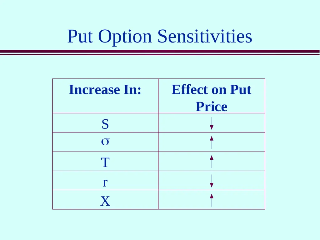
Put Option Sensitivities<br>
40
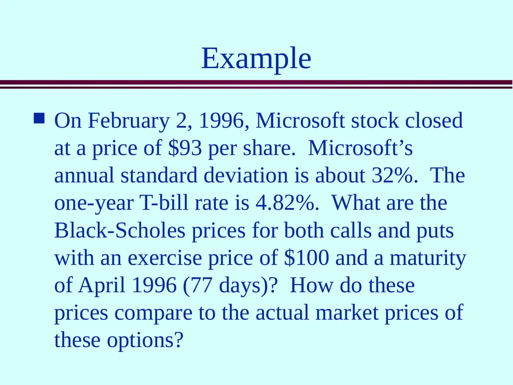
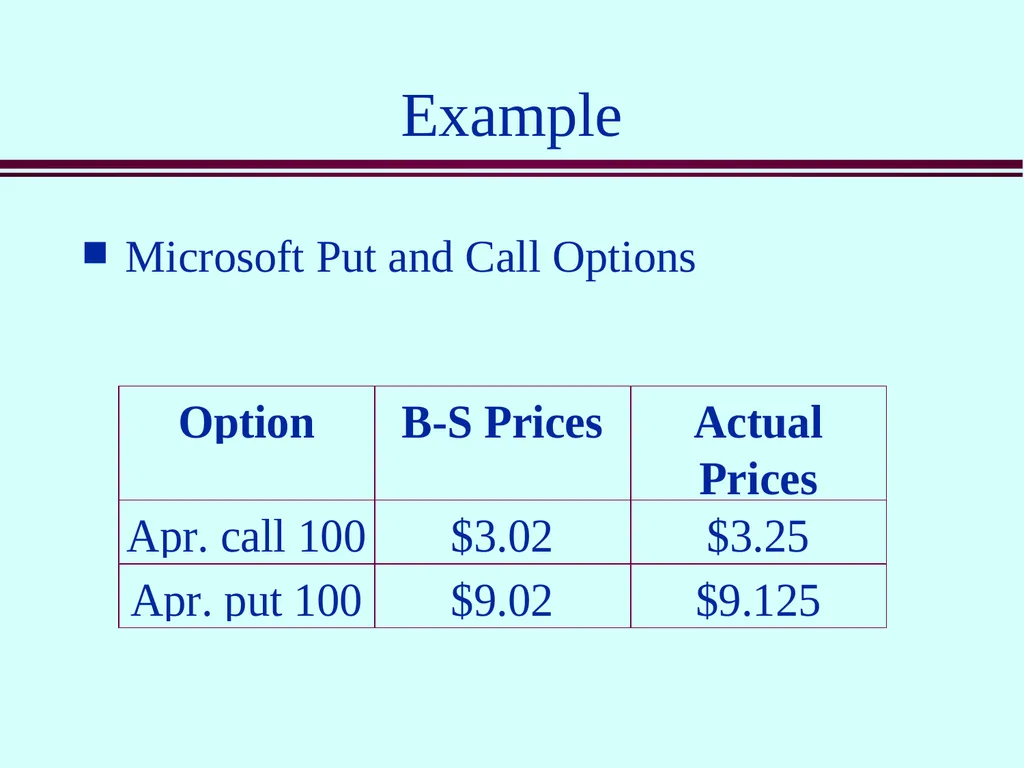
Example On February 2, 1996, Microsoft stock closed at a price of $93 per share. Microsoft’s annual standard deviation is about 32%. The one-year T-bill rate is 4.82%. What are the Black-Scholes prices for both calls and puts with an exercise price of $100 and a maturity of April 1996 (77 days)? How do these prices compare to the actual market prices of these options?<br>
41
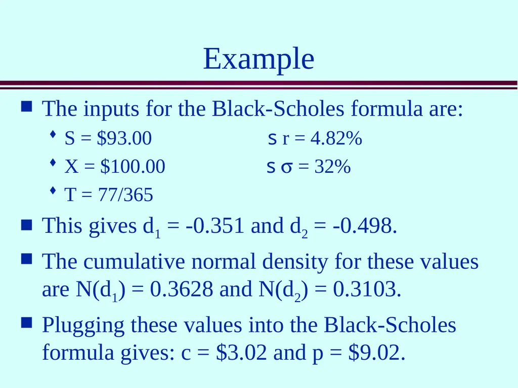
Example The inputs for the Black-Scholes formula are:
S = $93.00 s r = 4.82%
X = $100.00 s s = 32%
T = 77/365
This gives d1 = -0.351 and d2 = -0.498.
The cumulative normal density for these values are N(d1) = 0.3628 and N(d2) = 0.3103.
Plugging these values into the Black-Scholes formula gives: c = $3.02 and p = $9.02.<br>
S = $93.00 s r = 4.82%
X = $100.00 s s = 32%
T = 77/365
This gives d1 = -0.351 and d2 = -0.498.
The cumulative normal density for these values are N(d1) = 0.3628 and N(d2) = 0.3103.
Plugging these values into the Black-Scholes formula gives: c = $3.02 and p = $9.02.<br>
42
Example Microsoft Put and Call Options<br>
43
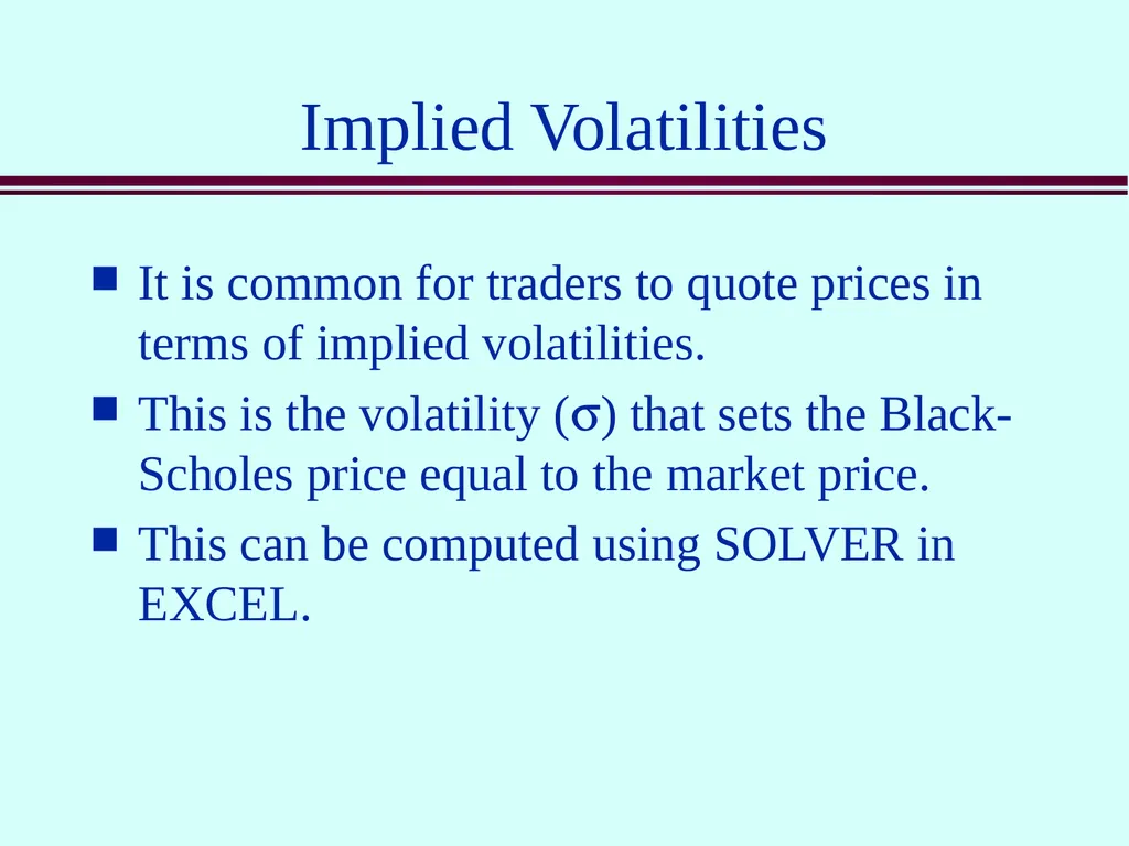
Implied Volatilities It is common for traders to quote prices in terms of implied volatilities.
This is the volatility (s) that sets the Black-Scholes price equal to the market price.
This can be computed using SOLVER in EXCEL.<br>
This is the volatility (s) that sets the Black-Scholes price equal to the market price.
This can be computed using SOLVER in EXCEL.<br>
44
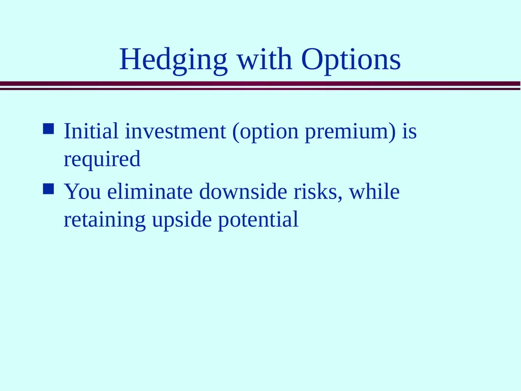
Hedging with Options Initial investment (option premium) is required
You eliminate downside risks, while retaining upside potential<br>
You eliminate downside risks, while retaining upside potential<br>
45
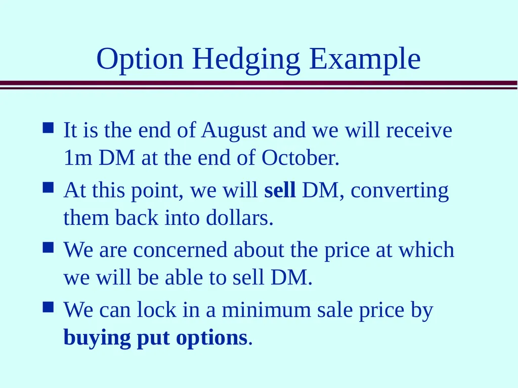
Option Hedging Example It is the end of August and we will receive 1m DM at the end of October.
At this point, we will sell DM, converting them back into dollars.
We are concerned about the price at which we will be able to sell DM.
We can lock in a minimum sale price by buying put options.<br>
At this point, we will sell DM, converting them back into dollars.
We are concerned about the price at which we will be able to sell DM.
We can lock in a minimum sale price by buying put options.<br>
46
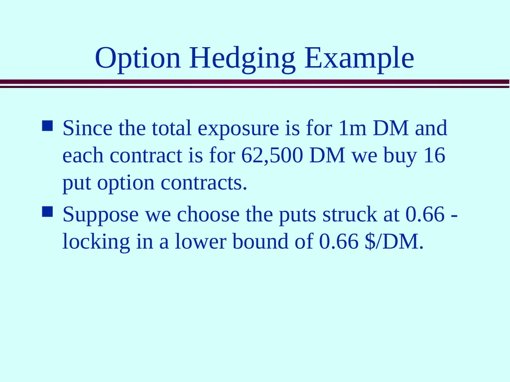
Option Hedging Example Since the total exposure is for 1m DM and each contract is for 62,500 DM we buy 16 put option contracts.
Suppose we choose the puts struck at 0.66 - locking in a lower bound of 0.66 $/DM.<br>
Suppose we choose the puts struck at 0.66 - locking in a lower bound of 0.66 $/DM.<br>
47
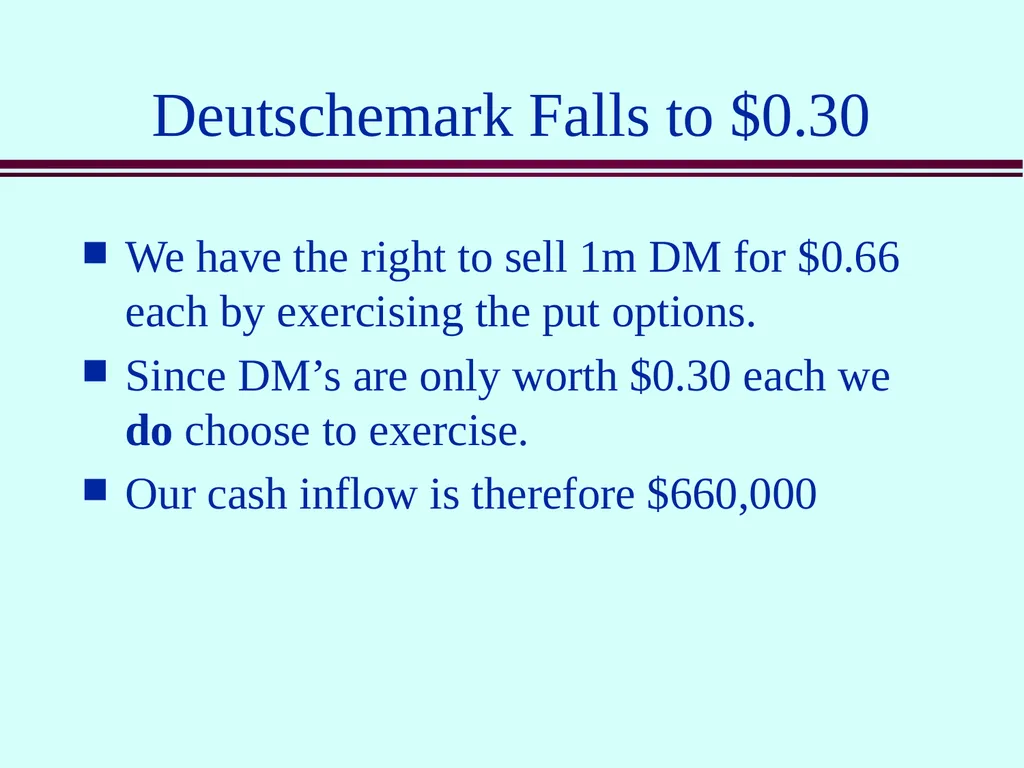
Deutschemark Falls to $0.30 We have the right to sell 1m DM for $0.66 each by exercising the put options.
Since DM’s are only worth $0.30 each we do choose to exercise.
Our cash inflow is therefore $660,000<br>
Since DM’s are only worth $0.30 each we do choose to exercise.
Our cash inflow is therefore $660,000<br>
48
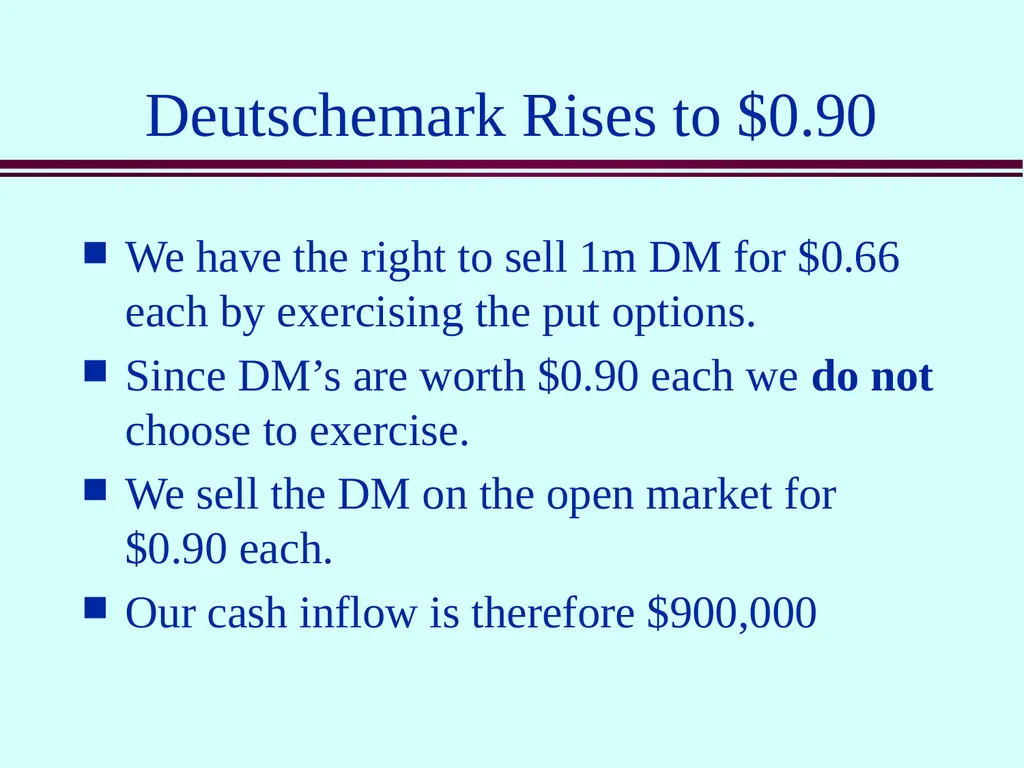
Deutschemark Rises to $0.90 We have the right to sell 1m DM for $0.66 each by exercising the put options.
Since DM’s are worth $0.90 each we do not choose to exercise.
We sell the DM on the open market for $0.90 each.
Our cash inflow is therefore $900,000<br>
Since DM’s are worth $0.90 each we do not choose to exercise.
We sell the DM on the open market for $0.90 each.
Our cash inflow is therefore $900,000<br>
49
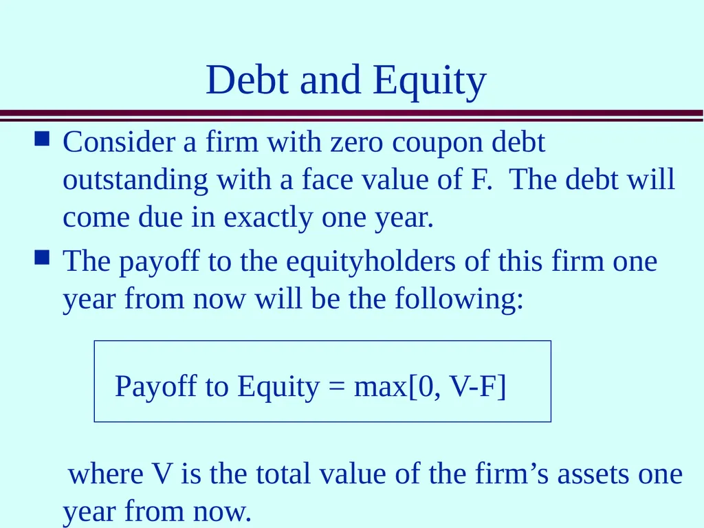
Debt and Equity Consider a firm with zero coupon debt outstanding with a face value of F. The debt will come due in exactly one year.
The payoff to the equityholders of this firm one year from now will be the following:
Payoff to Equity = max[0, V-F]
where V is the total value of the firm’s assets one year from now.<br>
The payoff to the equityholders of this firm one year from now will be the following:
Payoff to Equity = max[0, V-F]
where V is the total value of the firm’s assets one year from now.<br>
50
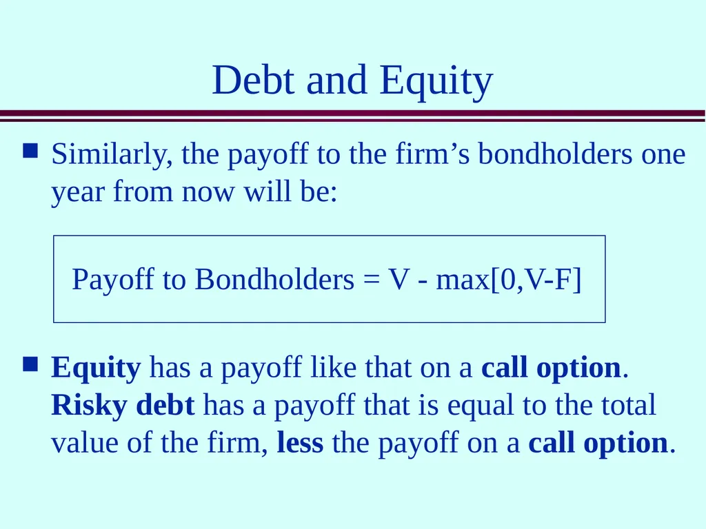
Debt and Equity Similarly, the payoff to the firm’s bondholders one year from now will be:
Payoff to Bondholders = V - max[0,V-F]
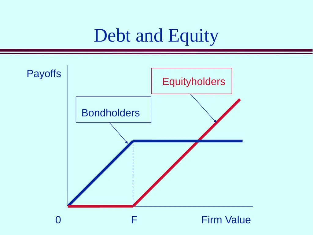
Equity has a payoff like that on a call option. Risky debt has a payoff that is equal to the total value of the firm, less the payoff on a call option.<br>
Payoff to Bondholders = V - max[0,V-F]
Equity has a payoff like that on a call option. Risky debt has a payoff that is equal to the total value of the firm, less the payoff on a call option.<br>
51
Debt and Equity Payoffs Firm Value 0 Equityholders Bondholders F<br>
52
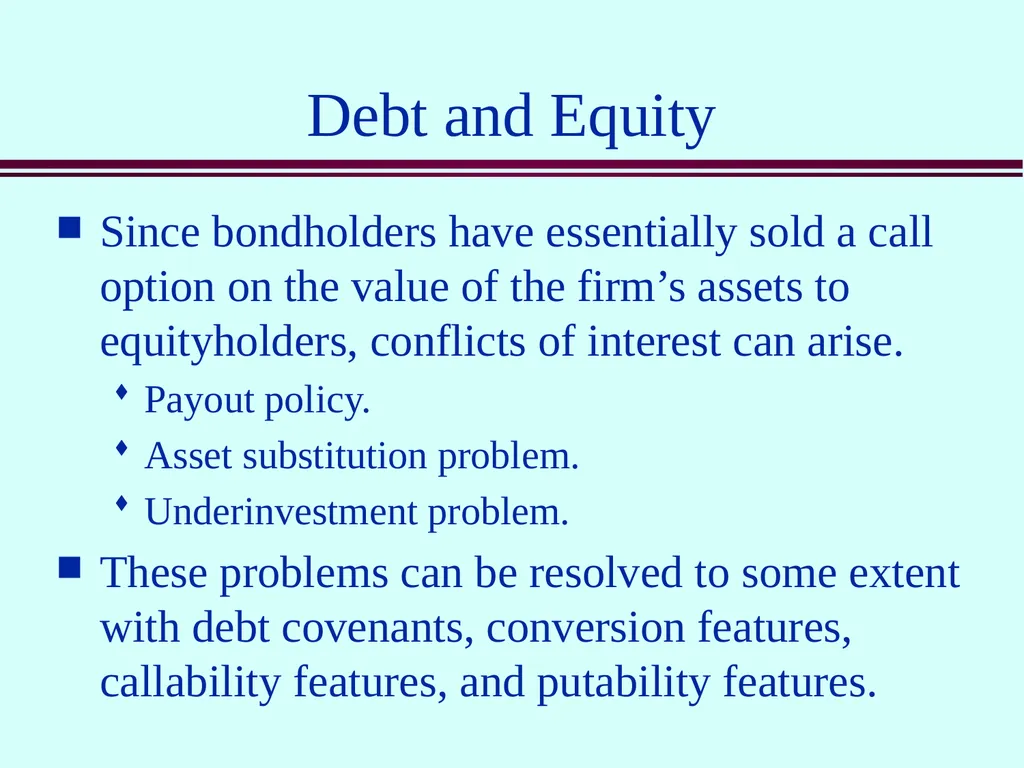
Debt and Equity Since bondholders have essentially sold a call option on the value of the firm’s assets to equityholders, conflicts of interest can arise.
Payout policy.
Asset substitution problem.
Underinvestment problem.
These problems can be resolved to some extent with debt covenants, conversion features, callability features, and putability features.<br>
Payout policy.
Asset substitution problem.
Underinvestment problem.
These problems can be resolved to some extent with debt covenants, conversion features, callability features, and putability features.<br>