Conducting interrupted time-series analysis for

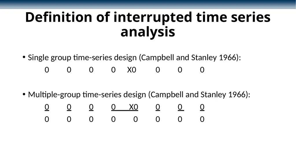
Definition of interrupted time series analysis Single group time-series design (Campbell and Stanley 1966):
0 0 0 0 X0 0 0 0

Multiple-group time-series design (Campbell and Stanley 1966):
0 0 0 0 X0 0 0 0
0 0 0 0 0 0 0 0<br>

When is ITSA useful Single-group ITSA:
For N-of-1 studies
When the only data available are summarized at the population-level (e.g. mortality or morbidity rates)
When observations are available for multiple evenly-spaced time points

Multiple-group ITSA:
Same as above but when a control group is available for comparison<br>

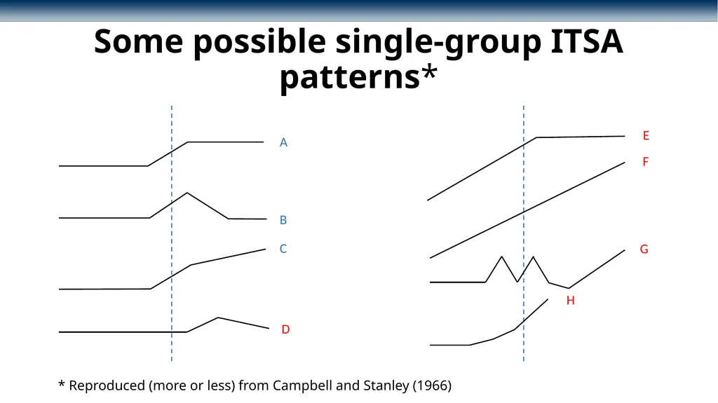
Some possible single-group ITSA patterns* * Reproduced (more or less) from Campbell and Stanley (1966) A B C D E F G H<br>

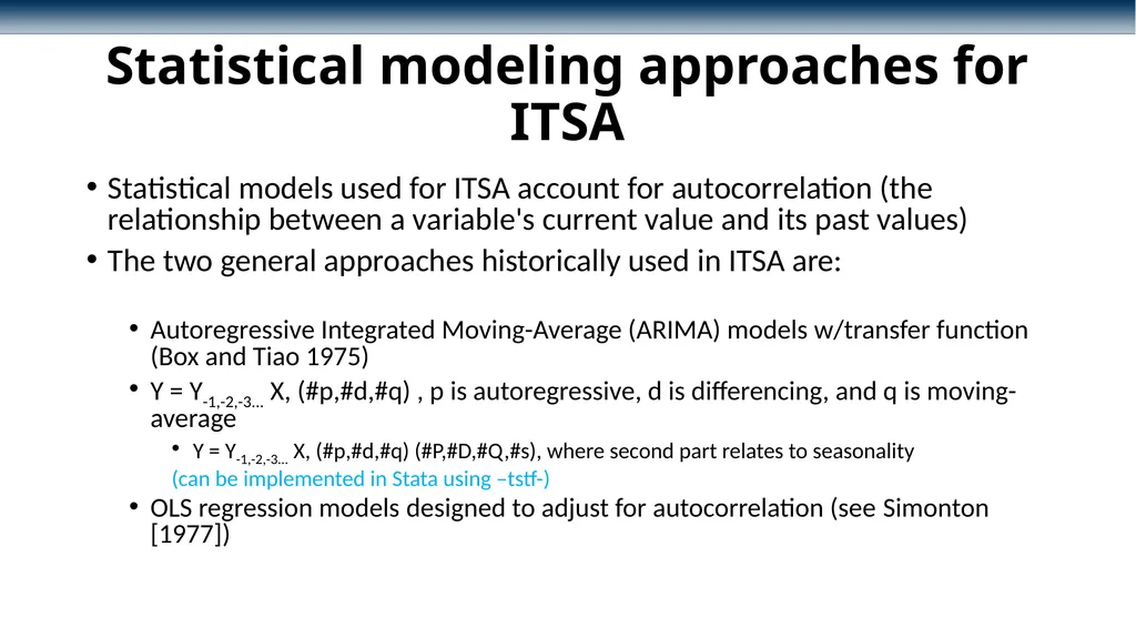
Statistical modeling approaches for ITSA Statistical models used for ITSA account for autocorrelation (the relationship between a variable's current value and its past values)
The two general approaches historically used in ITSA are:

Autoregressive Integrated Moving-Average (ARIMA) models w/transfer function (Box and Tiao 1975)
Y = Y-1,-2,-3... X, (#p,#d,#q) , p is autoregressive, d is differencing, and q is moving-average
Y = Y-1,-2,-3... X, (#p,#d,#q) (#P,#D,#Q,#s), where second part relates to seasonality
(can be implemented in Stata using –tstf-)
OLS regression models designed to adjust for autocorrelation (see Simonton [1977])<br>

Advantages of ARIMA Designed to handle autocorrelation, seasonality and cyclical trends
Non-linear models fit the data better than linear models<br>

Disadvantages of ARIMA At least 50, and preferably more than 100 observations are needed to stabilize the estimates (Box and Jenkins 1976)
ARIMA models are inherently designed for univariate time-series with a single intervention, not sequential interventions. Comparison to a control group is possible, but complicated
The procedural complexity of the methodology requires a great deal of expertise. Velicer and Harrop (1983) demonstrated that even highly trained researchers classified only 28 percent of computer-generated time series data correctly<br>

Advantages of OLS-ITSA models OLS may require as few as four observations (Simonton 1977)
OLS models are sufficiently flexible to accommodate multiple treatment periods and comparisons with one or more control groups
Post-estimation tests are available to assess whether the model correctly adjusted for autocorrelation
-lincom- can be used post-estimation to produce other estimates
OLS models can be used in conjunction with weighting or matching to improve causal inference
OLS models avoid the problems of model identification that encumbers the ARIMA methodology<br>

Disadvantages of OLS-ITSA models They produce linear estimates that may not fit the data well
Adjusting for seasonality and cyclical trends adds complexity to the modeling process<br>

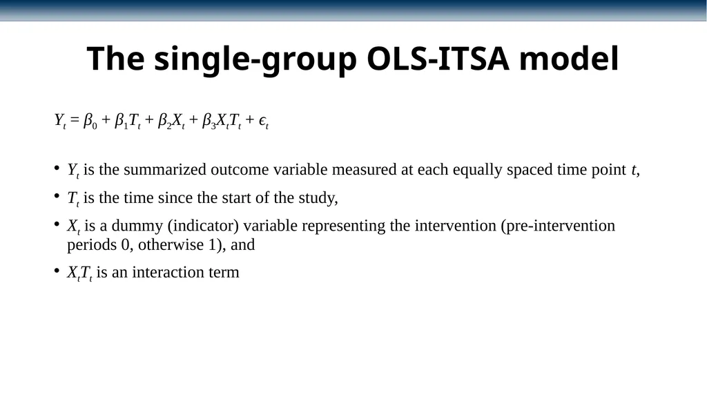
The single-group OLS-ITSA model Yt = β0 + β1Tt + β2Xt + β3XtTt + ϵt

Yt is the summarized outcome variable measured at each equally spaced time point t,
Tt is the time since the start of the study,
Xt is a dummy (indicator) variable representing the intervention (pre-intervention periods 0, otherwise 1), and
XtTt is an interaction term<br>

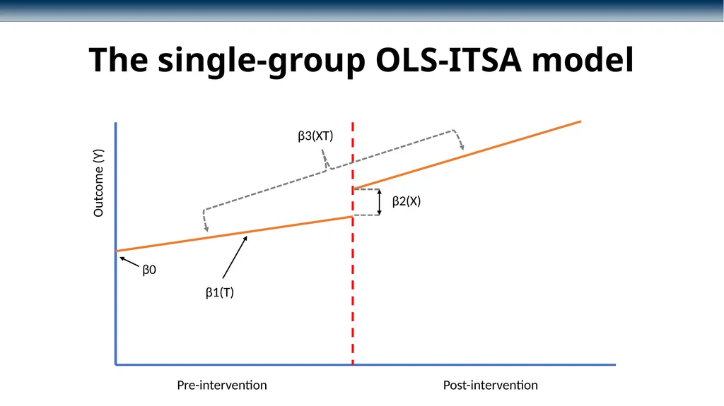
The single-group OLS-ITSA model Pre-intervention Post-intervention Outcome (Y) β0 β1(T) β2(X) β3(XT)<br>

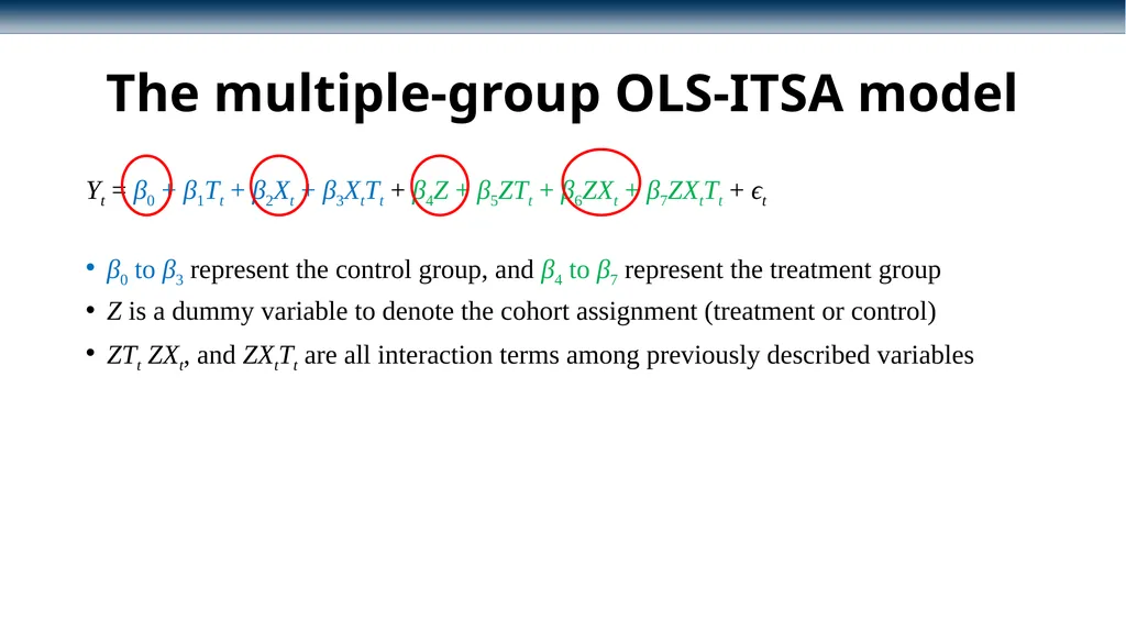
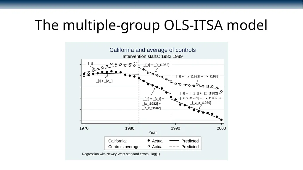
The multiple-group OLS-ITSA model Yt = β0 + β1Tt + β2Xt + β3XtTt + β4Z + β5ZTt + β6ZXt + β7ZXtTt + ϵt

β0 to β3 represent the control group, and β4 to β7 represent the treatment group
Z is a dummy variable to denote the cohort assignment (treatment or control)
ZTt ZXt, and ZXtTt are all interaction terms among previously described variables<br>

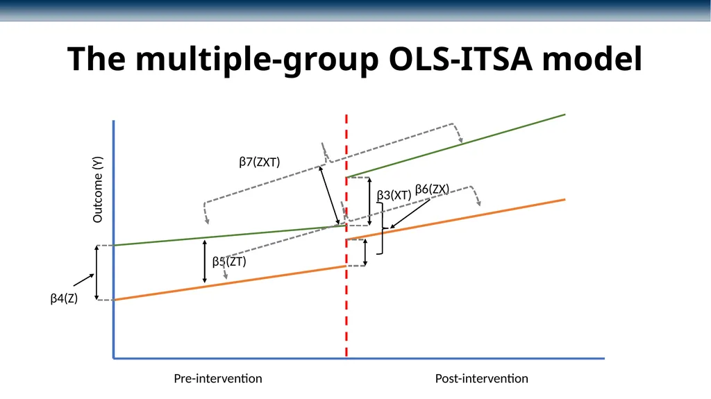
The multiple-group OLS-ITSA model Outcome (Y) Pre-intervention Post-intervention β4(Z) β5(ZT) β6(ZX) β7(ZXT) β3(XT)<br>

The multiple-group OLS-ITSA model<br>

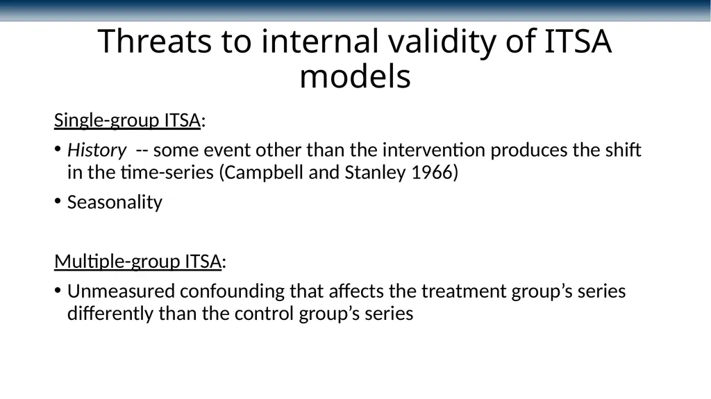
Threats to internal validity of ITSA models Single-group ITSA:
History -- some event other than the intervention produces the shift in the time-series (Campbell and Stanley 1966)
Seasonality

Multiple-group ITSA:
Unmeasured confounding that affects the treatment group’s series differently than the control group’s series<br>

Examples of where SG-ITSA results can be misinterpreted(math free)<br>

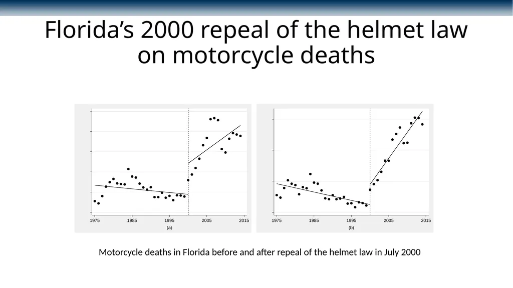
Florida’s 2000 repeal of the helmet law on motorcycle deaths Motorcycle deaths in Florida before and after repeal of the helmet law in July 2000<br>

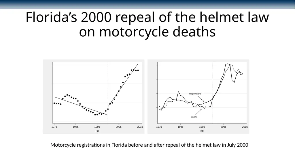
Florida’s 2000 repeal of the helmet law on motorcycle deaths Motorcycle registrations in Florida before and after repeal of the helmet law in July 2000<br>

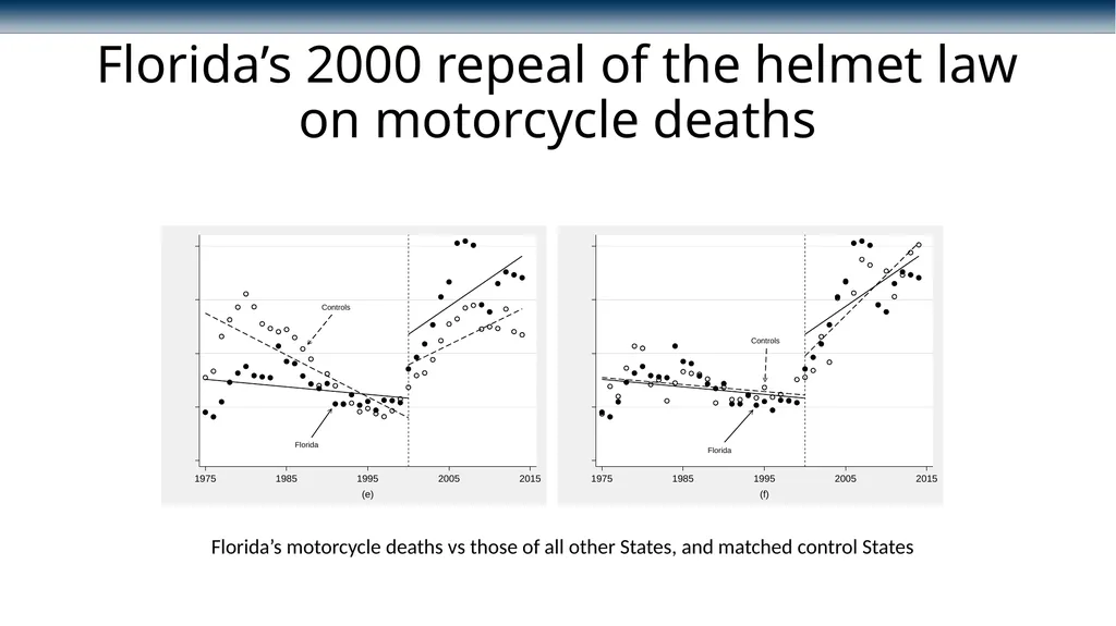
Florida’s 2000 repeal of the helmet law on motorcycle deaths Florida’s motorcycle deaths vs those of all other States, and matched control States<br>

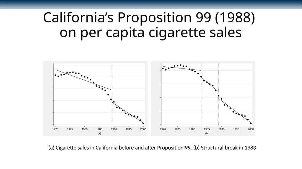
California’s Proposition 99 (1988) on per capita cigarette sales (a) Cigarette sales in California before and after Proposition 99. (b) Structural break in 1983<br>

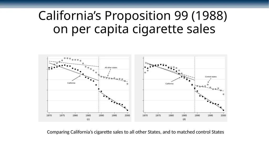
California’s Proposition 99 (1988) on per capita cigarette sales Comparing California’s cigarette sales to all other States, and to matched control States<br>

Louisiana’s repeals and reinstatements of the helmet law Louisiana’s multiple repeals/amendments/reinstatements of helmet law on motorcycle deaths<br>

Louisiana’s repeals and reinstatements of the helmet law Louisiana’s motorcycle deaths and registrations compared to all other States<br>

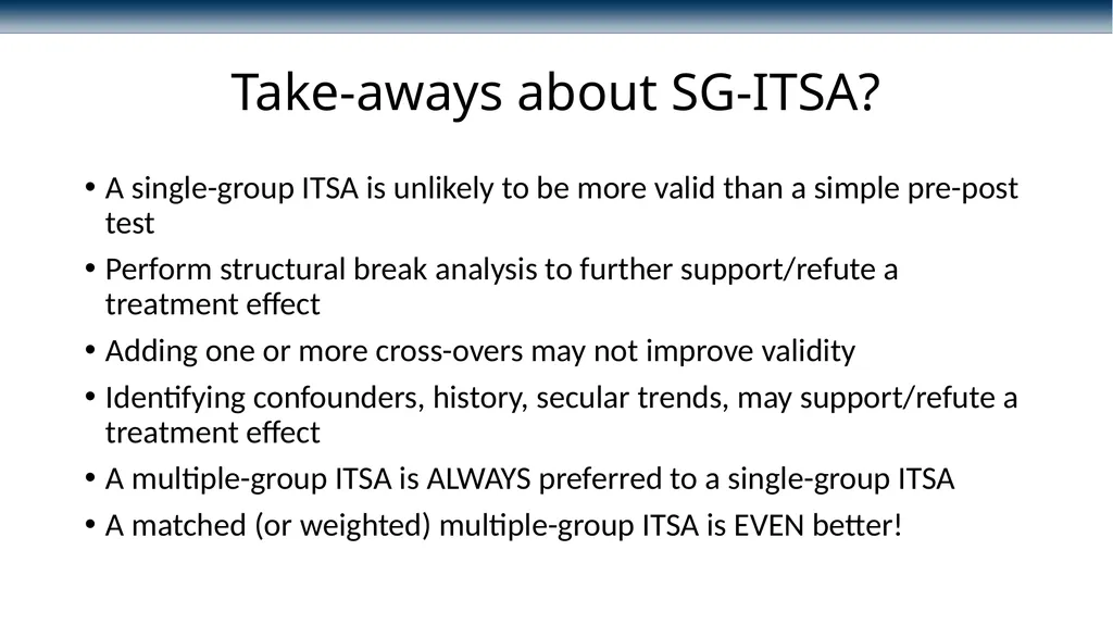
Take-aways about SG-ITSA? A single-group ITSA is unlikely to be more valid than a simple pre-post test
Perform structural break analysis to further support/refute a treatment effect
Adding one or more cross-overs may not improve validity
Identifying confounders, history, secular trends, may support/refute a treatment effect
A multiple-group ITSA is ALWAYS preferred to a single-group ITSA
A matched (or weighted) multiple-group ITSA is EVEN better!<br>

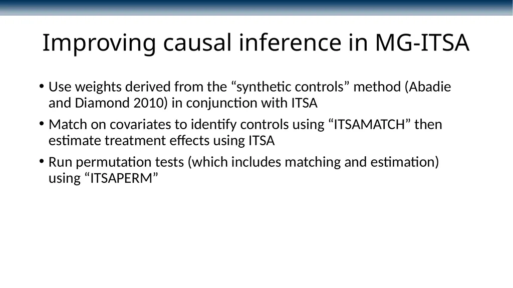
Improving causal inference in MG-ITSA Use weights derived from the “synthetic controls” method (Abadie and Diamond 2010) in conjunction with ITSA
Match on covariates to identify controls using “ITSAMATCH” then estimate treatment effects using ITSA
Run permutation tests (which includes matching and estimation) using “ITSAPERM”<br>

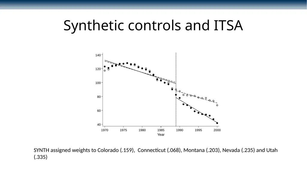
Synthetic controls and ITSA SYNTH assigned weights to Colorado (.159), Connecticut (.068), Montana (.203), Nevada (.235) and Utah (.335)<br>

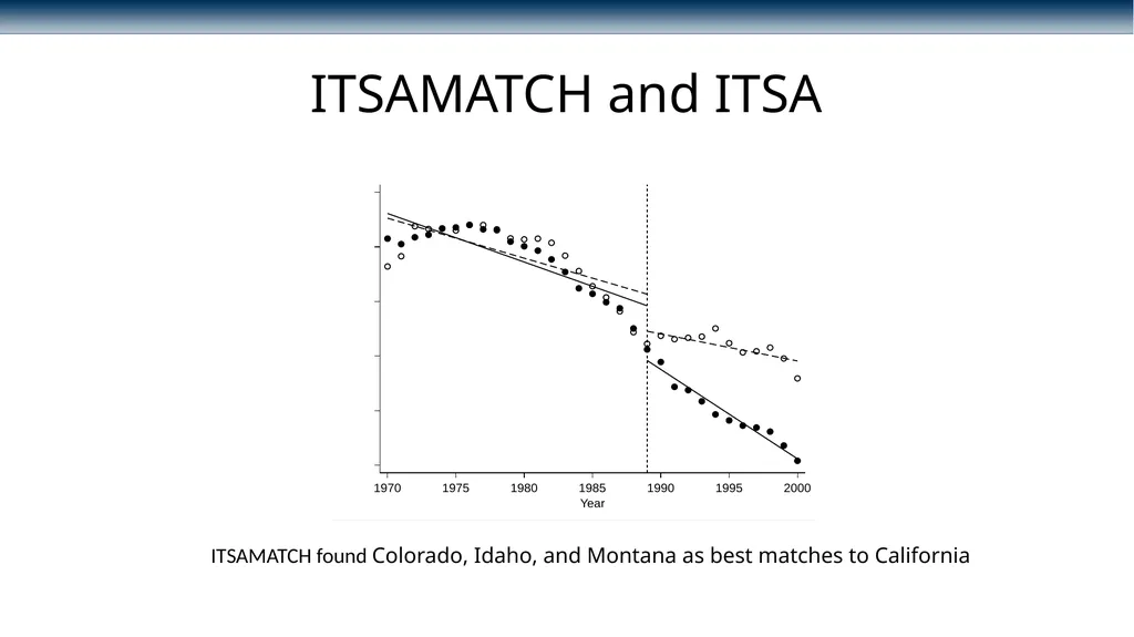
ITSAMATCH and ITSA ITSAMATCH found Colorado, Idaho, and Montana as best matches to California<br>

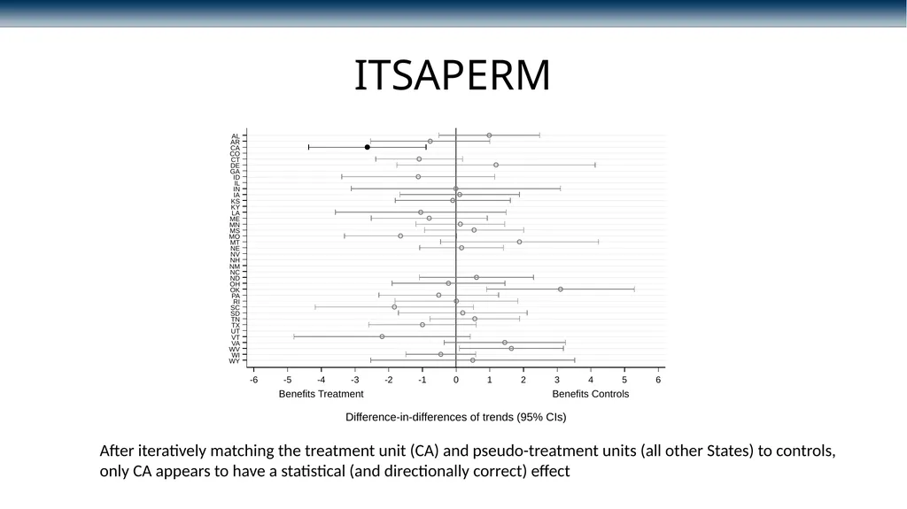
ITSAPERM After iteratively matching the treatment unit (CA) and pseudo-treatment units (all other States) to controls, only CA appears to have a statistical (and directionally correct) effect<br>

Conclusions Interrupted time series analysis is an observational (natural) study design that capitalizes on having many data-points for determining treatment effects (both visually and statistically)
A single-group ITSA may be no more valid than the simple pre-post design if some (non-observed) event other than the intervention produced the shift in the time-series
A multigroup ITSA that compares the treated unit to one or more comparable controls (via weighting or matching) is the most valid approach with observational data
Adding permutation tests provides an additional robustness check<br>

ITSA related packages for Stata ITSA – Performs interrupted time series analysis for single and multiple group comparisons
ITSAMATCH – Performs matching in multiple group interrupted time series analysis
ITSAPERM – Performs permutation tests for matched multiple group interrupted time series analysis
ITSARAND – Performs randomization tests for single-case and multiple-baseline AB phase designs 
XTITSA - Performs interrupted time series analysis with panel data<br>

References Abadie A, Diamond A. 2010. Synthetic control methods for comparative case studies: Estimating the effect of California's tobacco control program. J Am Stat Assoc. 105: 493‐505.
Box, G. E. P., and G. M. Jenkins. 1976. Time Series Analysis: Forecasting and Control. San Francisco, CA: Holden Day.
Box, G. E. P., and G. C. Tiao. 1975. Intervention analysis with applications to economic and environmental problems. Journal of the American Statistical Association 70: 70–79.
Campbell, D. T., and J. C. Stanley. 1966. Experimental and Quasi-Experimental Designs for Research. Chicago, IL: Rand McNally.
Linden A. 2015. Conducting interrupted time series analysis for single and multiple group comparisons. Stata Journal 15: 480-500.
Linden A. 2016. Challenges to validity in single-group interrupted time series analysis. Journal of Evaluation in Clinical Practice 23: 413–418.
Linden A. 2017. A comprehensive set of post-estimation measures to enrich interrupted time series analysis. Stata Journal 17: 73-88.
Linden A. 2017. Persistent threats to validity in single-group interrupted time series analysis with a crossover design. Journal of Evaluation in Clinical Practice 23: 419–425.
Linden A. 2018. A matching framework to improve causal inference in interrupted time series analysis. Journal of Evaluation in Clinical Practice 24: 408-415.
Linden A. 2018. Combining synthetic controls and interrupted time series analysis to improve causal inference in program evaluation. Journal of Evaluation in Clinical Practice 24: 447-453.
Linden A. 2018. Using permutation tests to enhance causal inference in interrupted time series analysis. Journal of Evaluation in Clinical Practice 24:496-501.
Linden A. 2022. Erratum: A comprehensive set of post-estimation measures to enrich interrupted time series analysis. Stata Journal 22:231-233.
Simonton, D. K. 1977. Cross-sectional time-series experiments: Some suggested statistical analyses. Psychological Bulletin 84: 489–502.
Velicer, W. F., and J. Harrop. 1983. The reliability and accuracy of time series model identification. Evaluation Review 7: 551–560.<br>

Thank You!<br>