
CS 106X, Lecture 23 Dijkstra and A* Search





Description: CS 106X, Lecture 23 Dijkstra and A Search reading: Programming Abstractions in C, Chapter 18 Plan For Today Recap: DFS and BFS Dijkstras Algorithm Announcements A Search Plan For Today Recap: DFS and BFS Dijkstras Algorithm
Related Topics
Download Presentation
"CS 106X, Lecture 23 Dijkstra and A* Search" is the property of its rightful owner. Permission is granted to download and print the materials on this website for personal, non-commercial use only, and to display it on your personal computer provided you do not modify the materials and that you retain all copyright notices contained in the materials. By downloading content from our website, you accept the terms of this agreement.
Presentation Transcript
slide1. CS 106X, Lecture 23
Dijkstra and A* Search reading:
Programming Abstractions in C++, Chapter 18<br>
slide2. Plan For Today Recap: DFS and BFS
Dijkstra’s Algorithm
Announcements
A* Search<br>
slide3. Plan For Today Recap: DFS and BFS
Dijkstra’s Algorithm
Announcements
A* Search<br>
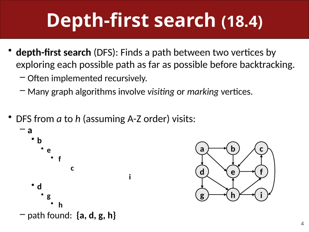
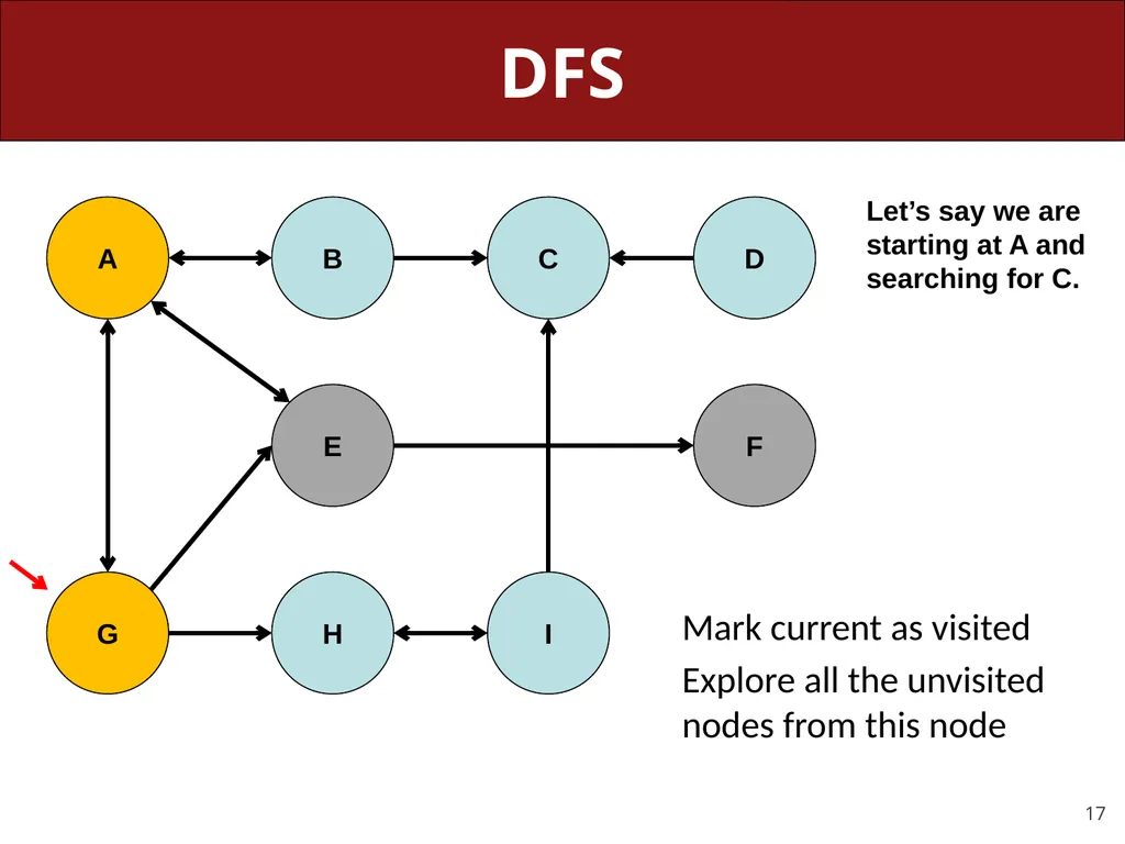
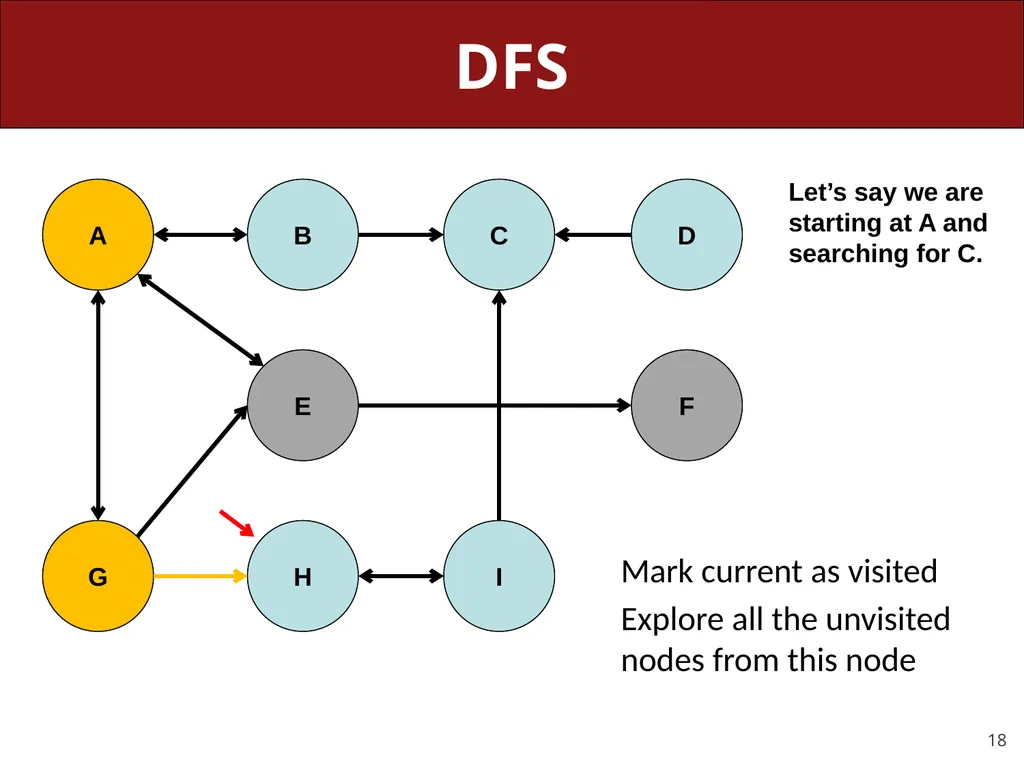
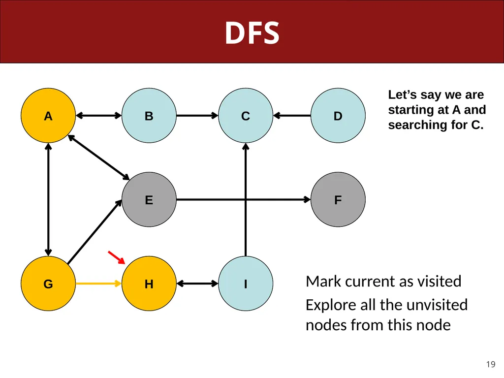
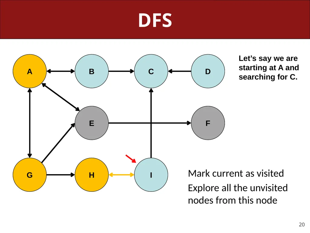
slide4. Depth-first search (18.4) depth-first search (DFS): Finds a path between two vertices by exploring each possible path as far as possible before backtracking.
Often implemented recursively.
Many graph algorithms involve visiting or marking vertices.
DFS from a to h (assuming A-Z order) visits:
a
b
e
f
c
i
d
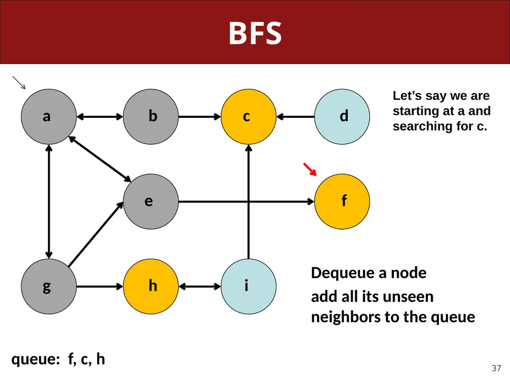
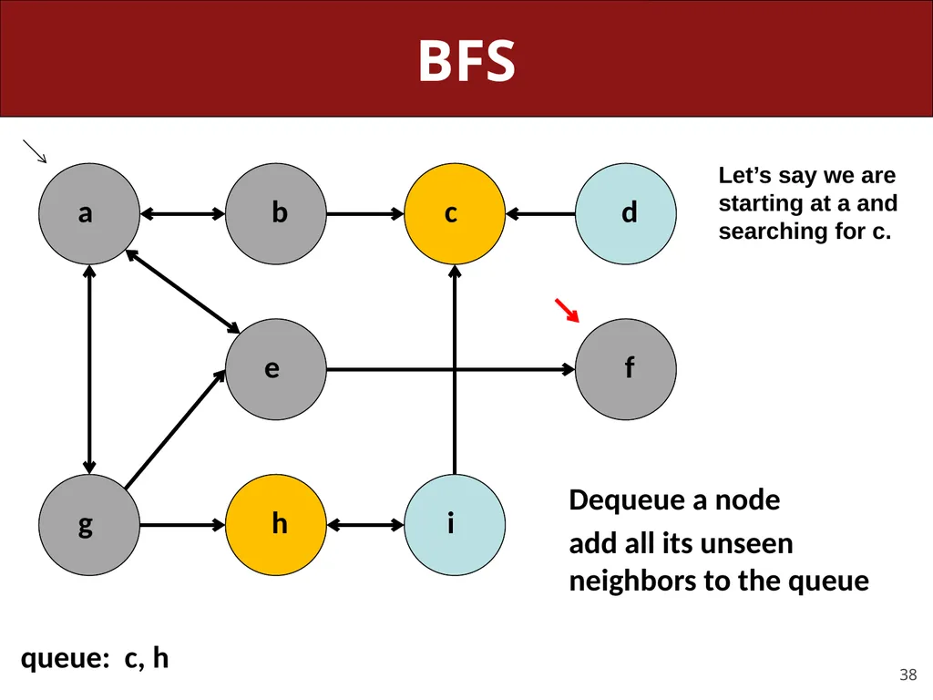
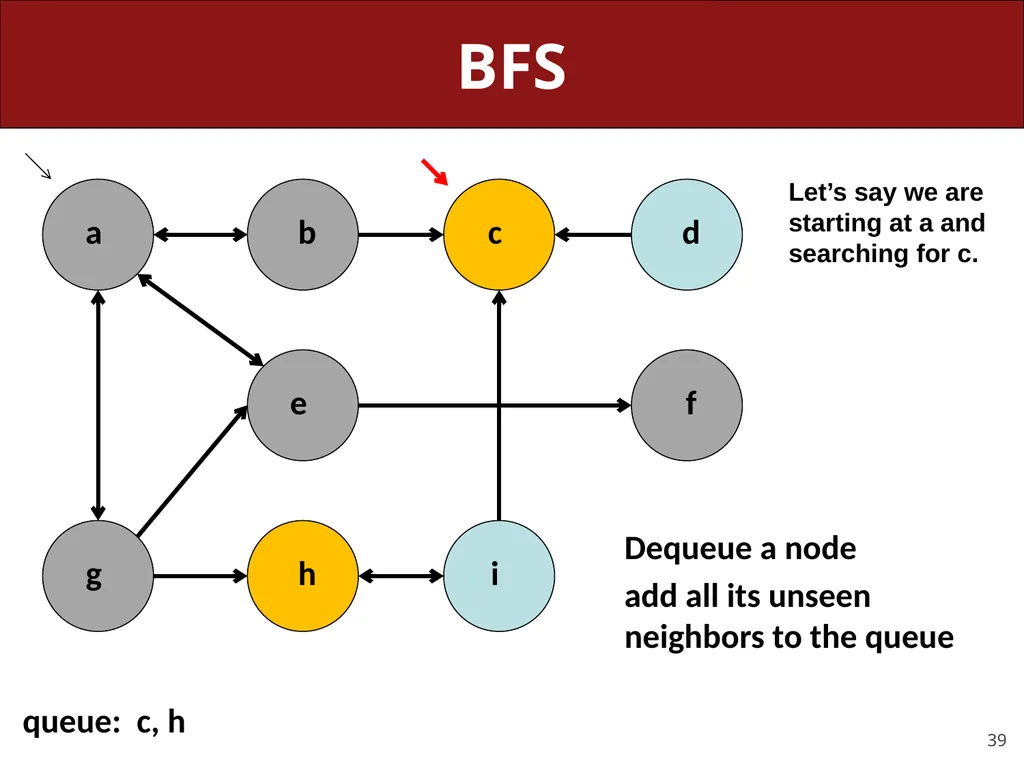
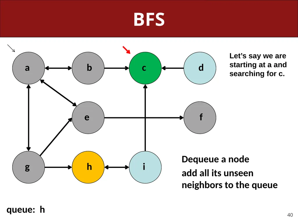
g
h
path found: {a, d, g, h}<br>
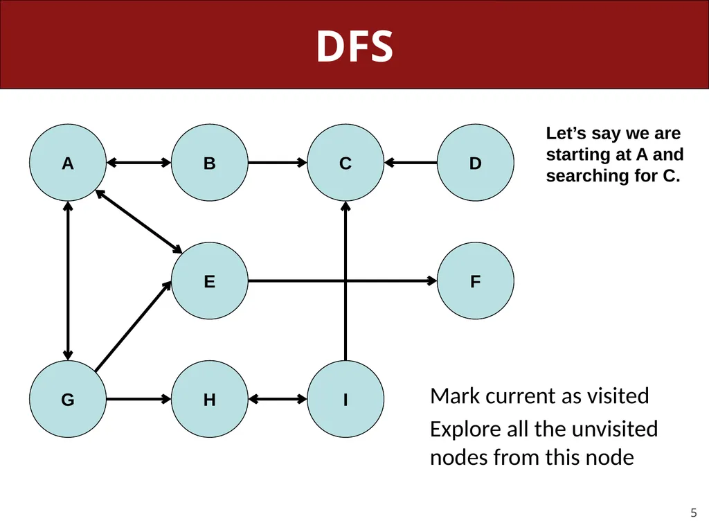
slide5. DFS Mark current as visited
Explore all the unvisited nodes from this node A B C D F E I H G Let’s say we are starting at A and searching for C.<br>
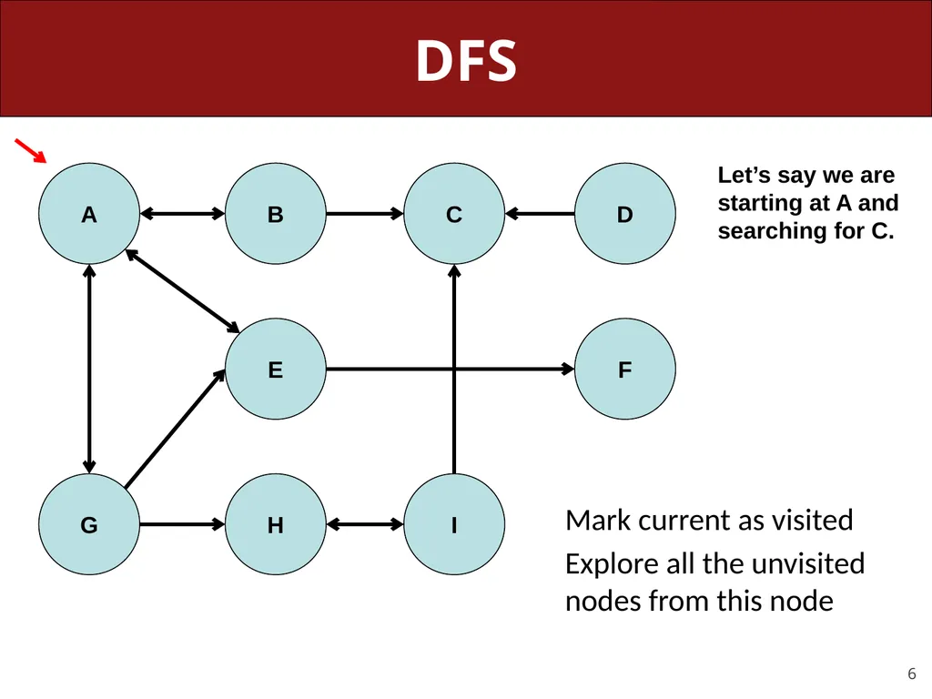
slide6. DFS Mark current as visited
Explore all the unvisited nodes from this node A B C D F E I H G Let’s say we are starting at A and searching for C.<br>
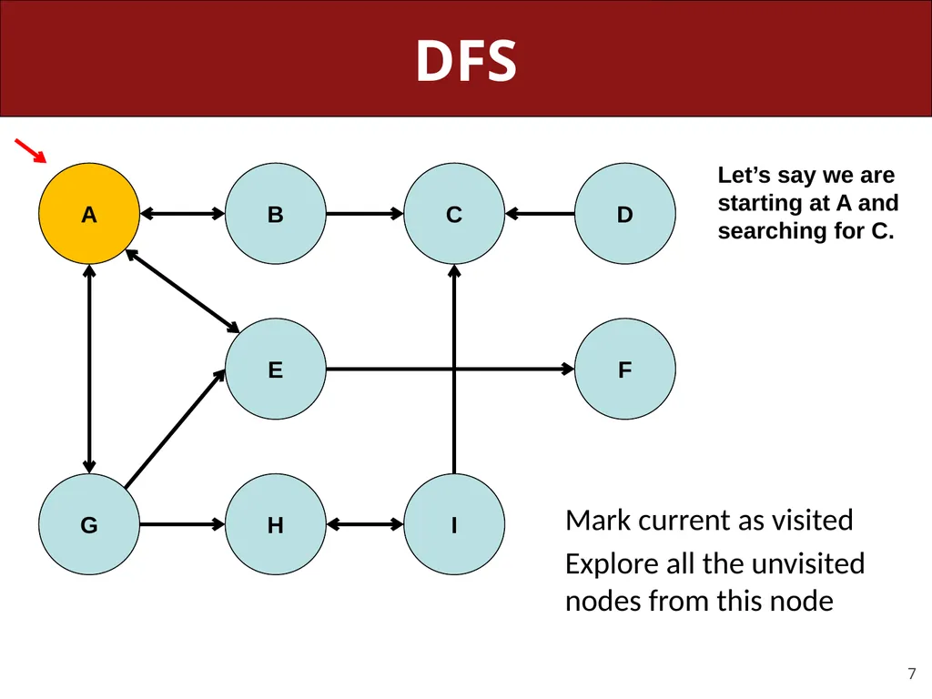
slide7. DFS Mark current as visited
Explore all the unvisited nodes from this node A B C D F E I H G Let’s say we are starting at A and searching for C.<br>
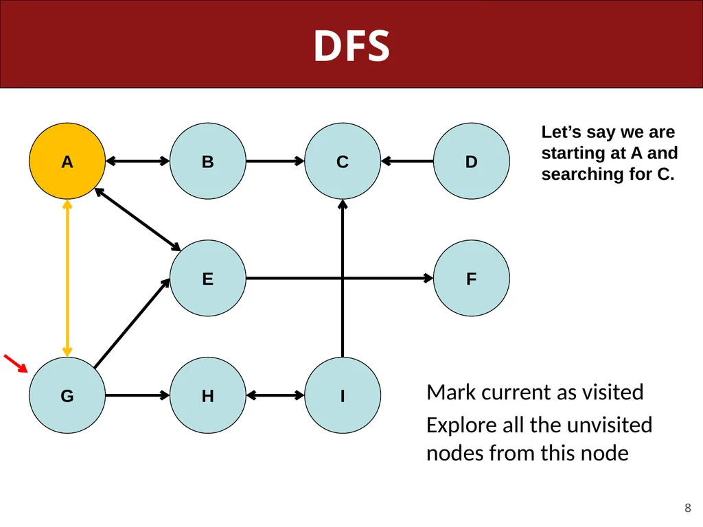
slide8. DFS Mark current as visited
Explore all the unvisited nodes from this node A B C D F E I H G Let’s say we are starting at A and searching for C.<br>
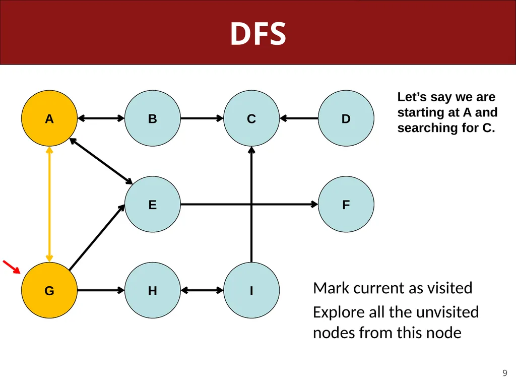
slide9. DFS Mark current as visited
Explore all the unvisited nodes from this node A B C D F E I H G Let’s say we are starting at A and searching for C.<br>
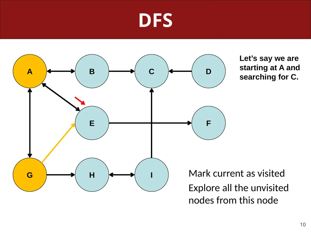
slide10. DFS Mark current as visited
Explore all the unvisited nodes from this node A B C D F E I H G Let’s say we are starting at A and searching for C.<br>
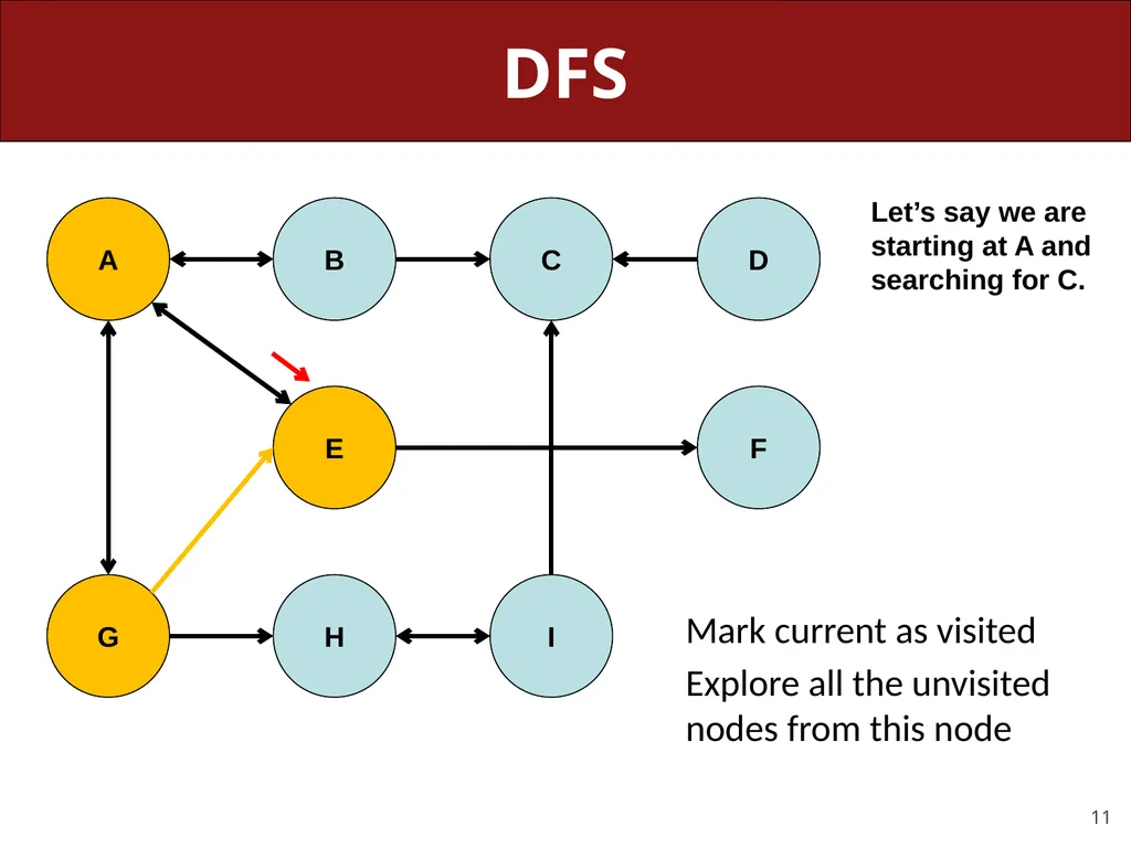
slide11. DFS Mark current as visited
Explore all the unvisited nodes from this node A B C D F E I H G Let’s say we are starting at A and searching for C.<br>
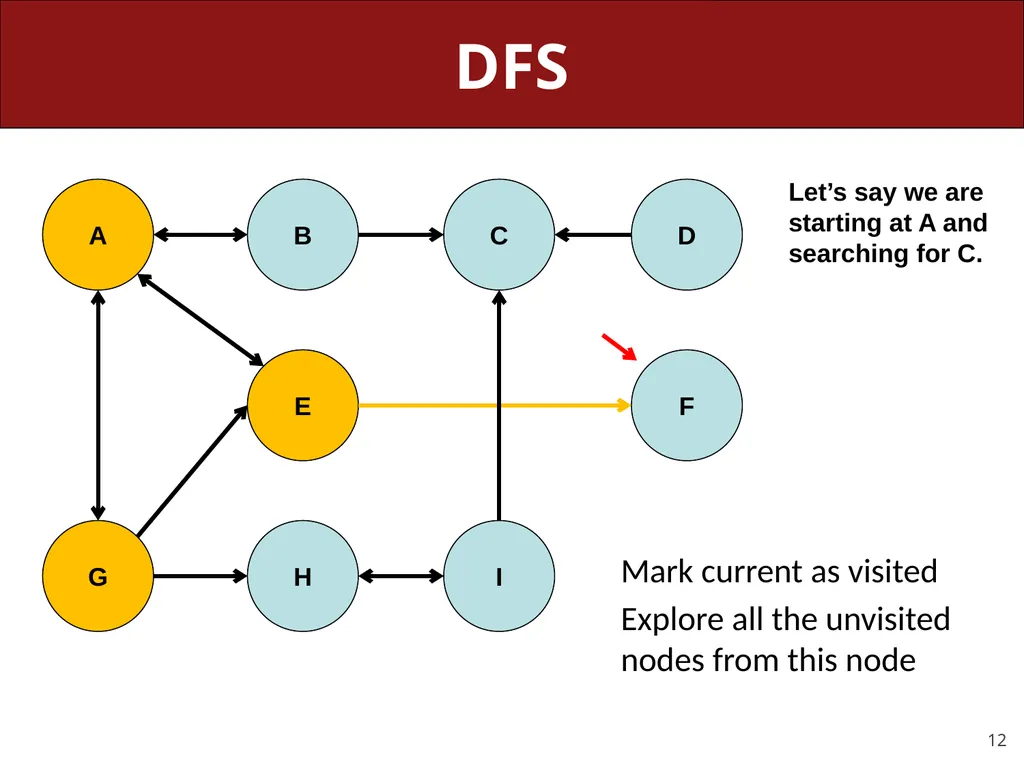
slide12. DFS Mark current as visited
Explore all the unvisited nodes from this node A B C D F E I H G Let’s say we are starting at A and searching for C.<br>
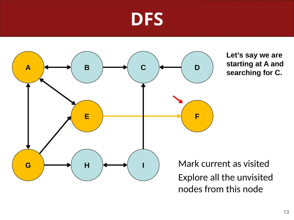
slide13. DFS Mark current as visited
Explore all the unvisited nodes from this node A B C D F E I H G Let’s say we are starting at A and searching for C.<br>
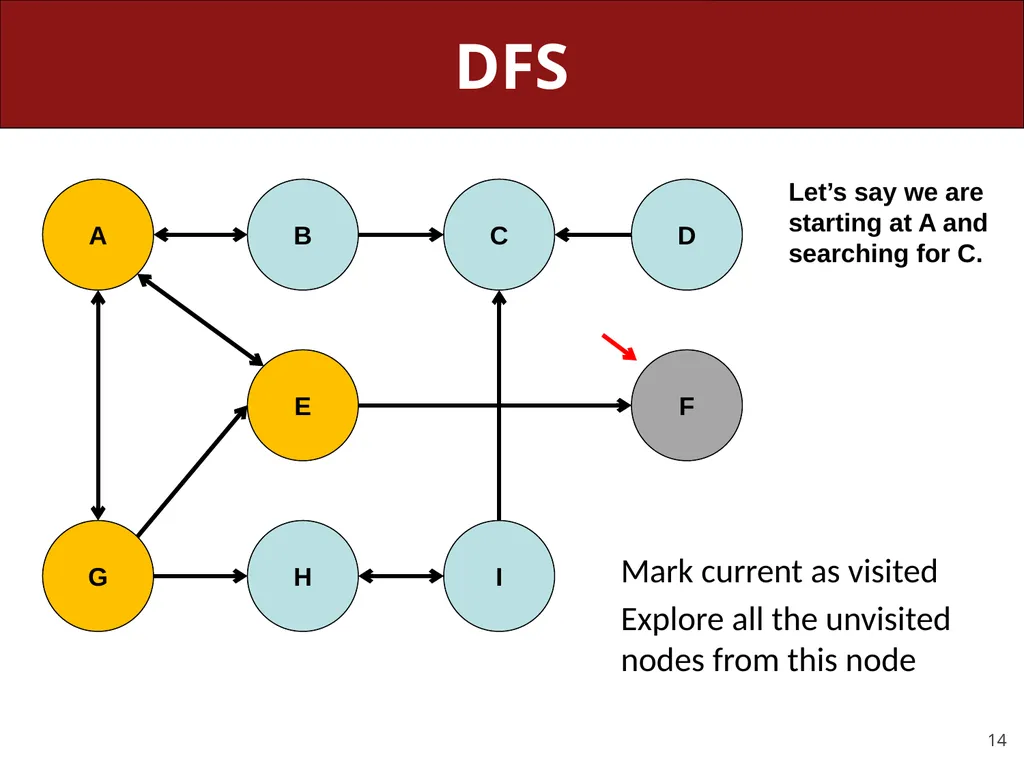
slide14. DFS Mark current as visited
Explore all the unvisited nodes from this node A B C D F E I H G Let’s say we are starting at A and searching for C.<br>
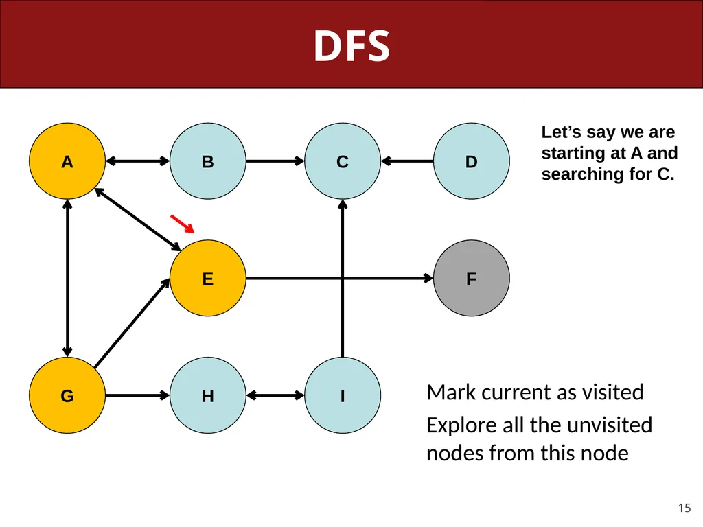
slide15. DFS Mark current as visited
Explore all the unvisited nodes from this node A B C D F E I H G Let’s say we are starting at A and searching for C.<br>
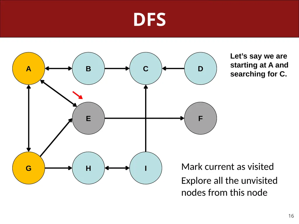
slide16. DFS Mark current as visited
Explore all the unvisited nodes from this node A B C D F E I H G Let’s say we are starting at A and searching for C.<br>
slide17. DFS Mark current as visited
Explore all the unvisited nodes from this node A B C D F E I H G Let’s say we are starting at A and searching for C.<br>
slide18. DFS Mark current as visited
Explore all the unvisited nodes from this node A B C D F E I H G Let’s say we are starting at A and searching for C.<br>
slide19. DFS Mark current as visited
Explore all the unvisited nodes from this node A B C D F E I H G Let’s say we are starting at A and searching for C.<br>
slide20. DFS Mark current as visited
Explore all the unvisited nodes from this node A B C D F E I H G Let’s say we are starting at A and searching for C.<br>
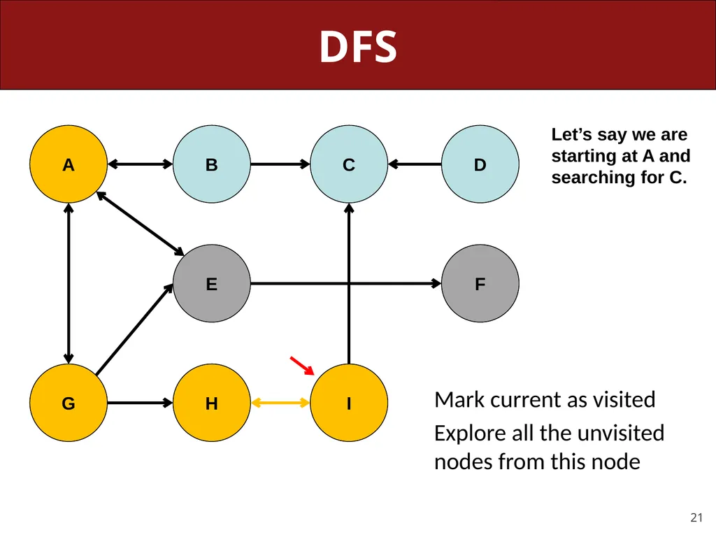
slide21. DFS Mark current as visited
Explore all the unvisited nodes from this node A B C D F E I H G Let’s say we are starting at A and searching for C.<br>
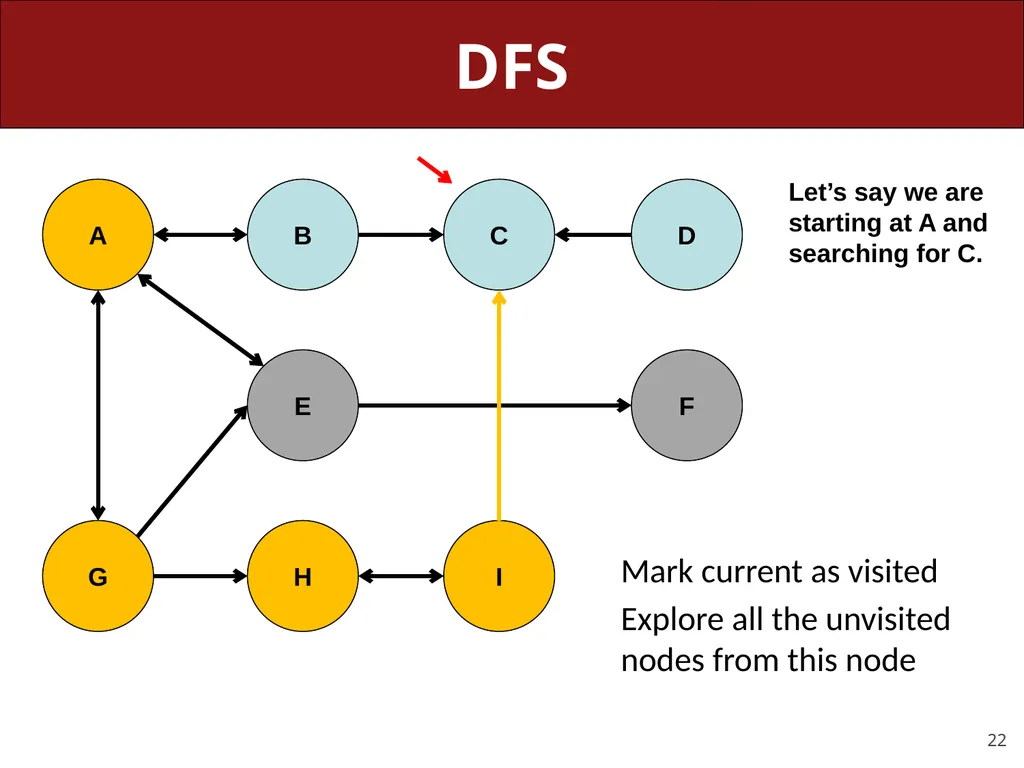
slide22. DFS Mark current as visited
Explore all the unvisited nodes from this node A B C D F E I H G Let’s say we are starting at A and searching for C.<br>
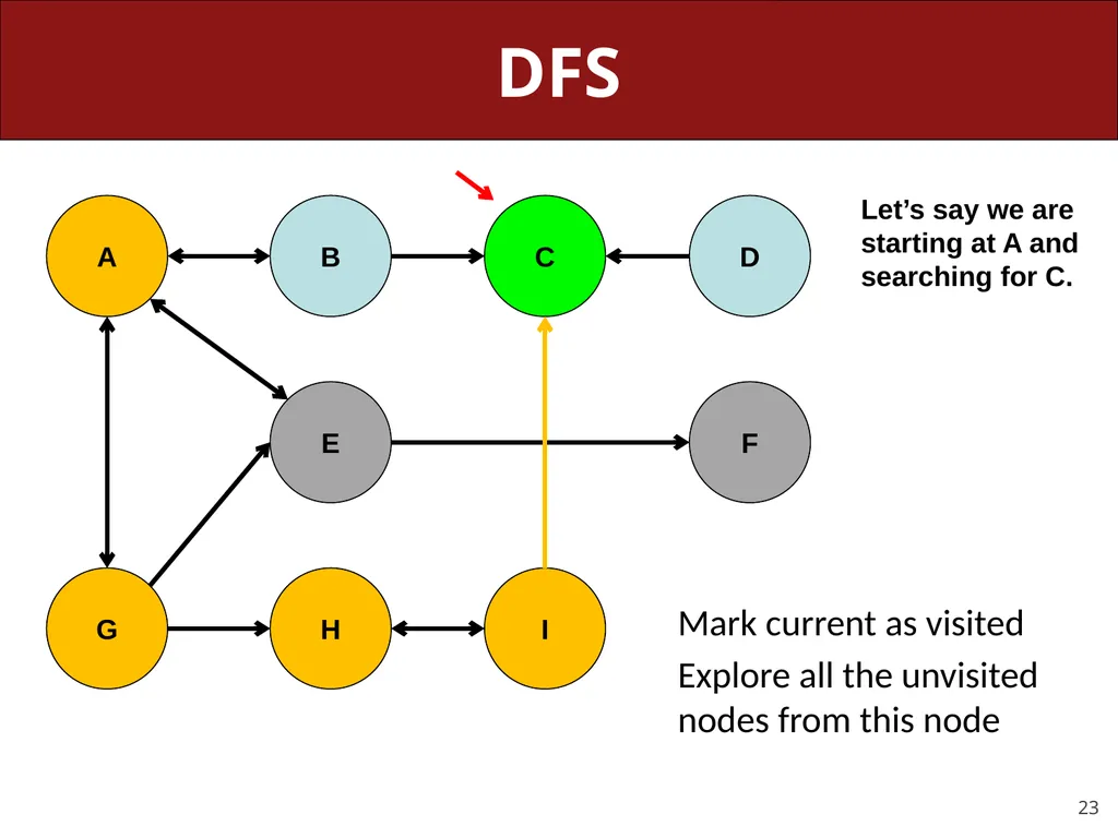
slide23. DFS Mark current as visited
Explore all the unvisited nodes from this node A B C D F E I H G Let’s say we are starting at A and searching for C.<br>
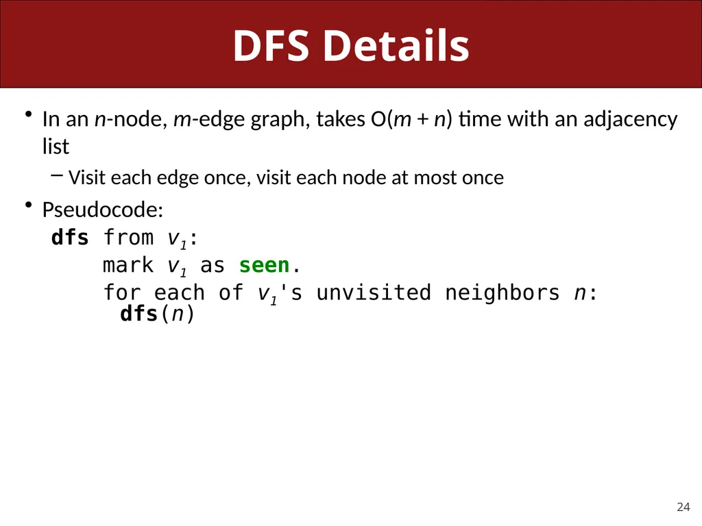
slide24. DFS Details In an n-node, m-edge graph, takes O(m + n) time with an adjacency list
Visit each edge once, visit each node at most once
Pseudocode:
dfs from v1:
mark v1 as seen.
for each of v1's unvisited neighbors n: dfs(n)<br>
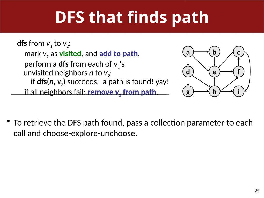
slide25. DFS that finds path dfs from v1 to v2:
mark v1 as visited, and add to path.
perform a dfs from each of v1's unvisited neighbors n to v2: if dfs(n, v2) succeeds: a path is found! yay!
if all neighbors fail: remove v1 from path.
To retrieve the DFS path found, pass a collection parameter to each call and choose-explore-unchoose.<br>
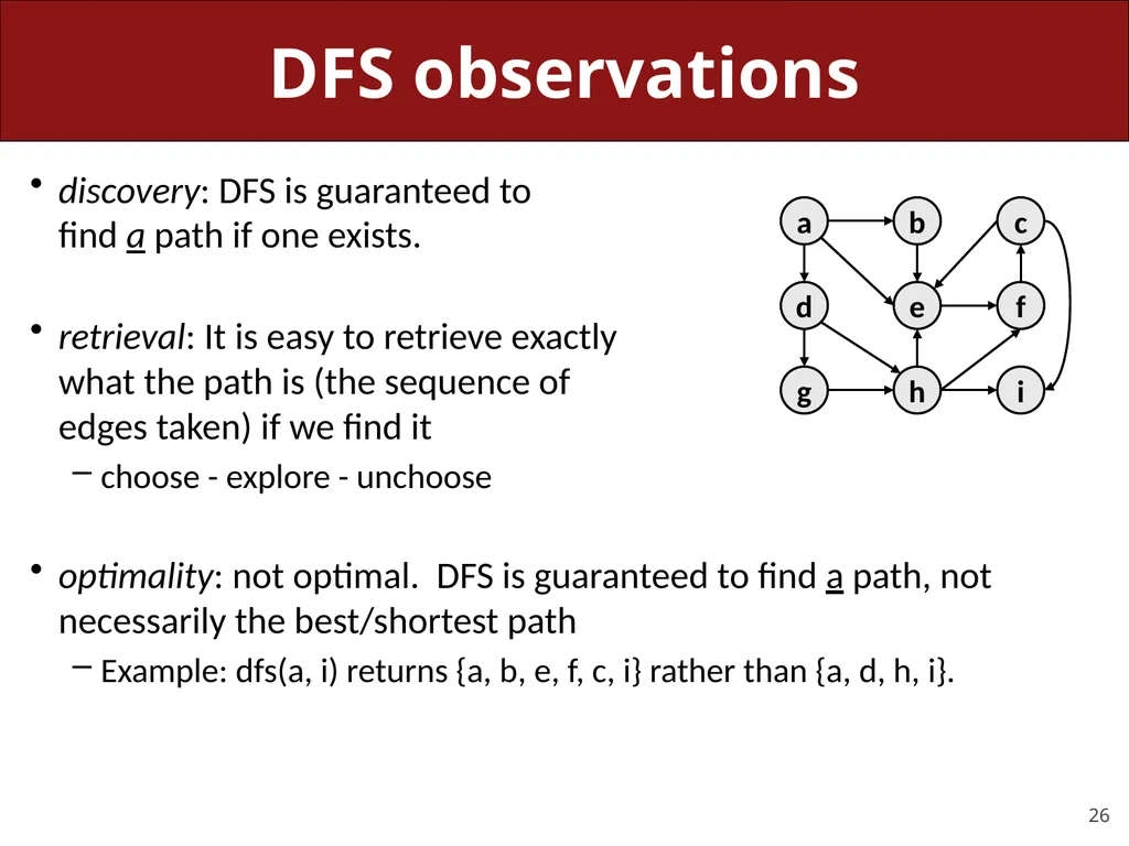
slide26. DFS observations discovery: DFS is guaranteed to find a path if one exists.
retrieval: It is easy to retrieve exactly what the path is (the sequence of edges taken) if we find it
choose - explore - unchoose
optimality: not optimal. DFS is guaranteed to find a path, not necessarily the best/shortest path
Example: dfs(a, i) returns {a, b, e, f, c, i} rather than {a, d, h, i}.<br>
slide27. Finding Shortest Paths We can find paths between two nodes, but how can we find the shortest path?
Fewest number of steps to complete a task?
Least amount of edits between two words?<br>
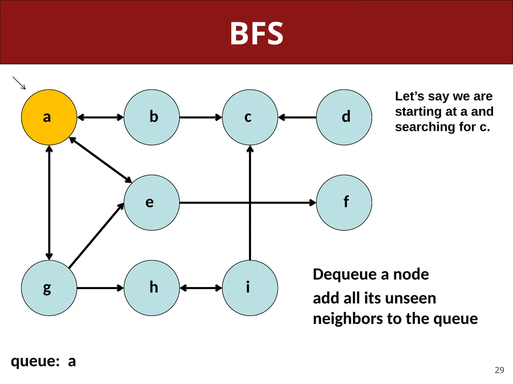
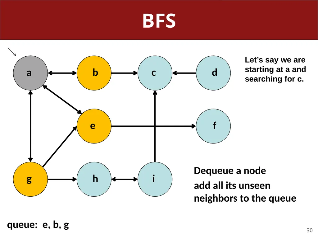
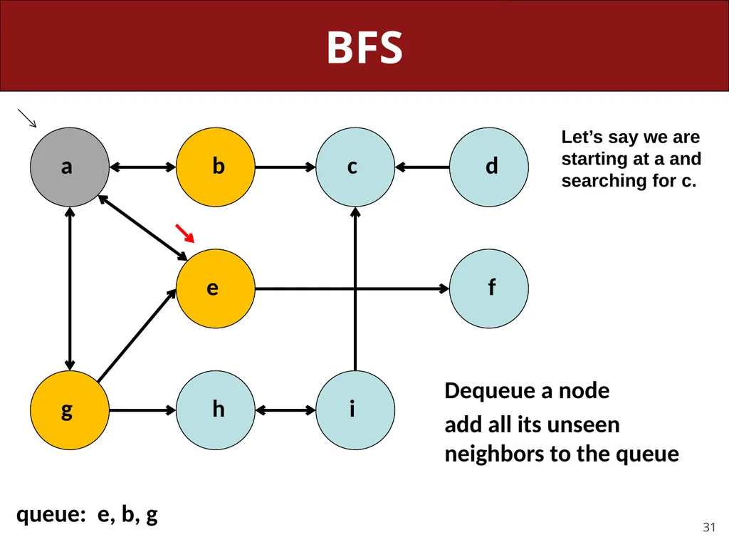
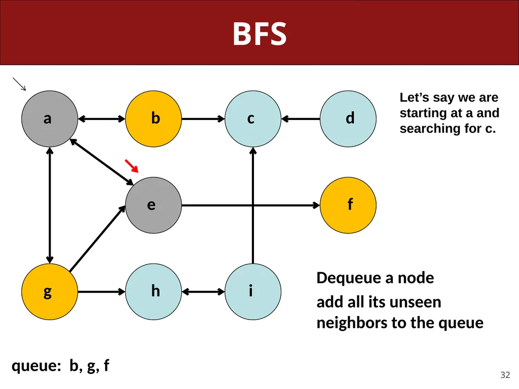
slide28. Breadth-First Search (BFS) Idea: processing a node involves knowing we need to visit all its neighbors (just like DFS)
Need to keep a TODO list of nodes to process
Keep a Queue of nodes as our TODO list
Idea: dequeue a node, enqueue all its neighbors
Still will return the same nodes as reachable, just might have shorter paths<br>
slide29. BFS a b c d f e g h i queue: a Dequeue a node
add all its unseen neighbors to the queue Let’s say we are starting at a and searching for c.<br>
slide30. BFS a b c d f e g h i queue: e, b, g Dequeue a node
add all its unseen neighbors to the queue Let’s say we are starting at a and searching for c.<br>
slide31. BFS a b c d f e g h i queue: e, b, g Dequeue a node
add all its unseen neighbors to the queue Let’s say we are starting at a and searching for c.<br>
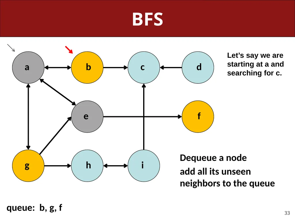
slide32. BFS a b c d f e g h i queue: b, g, f Dequeue a node
add all its unseen neighbors to the queue Let’s say we are starting at a and searching for c.<br>
slide33. BFS a b c d f e g h i queue: b, g, f Dequeue a node
add all its unseen neighbors to the queue Let’s say we are starting at a and searching for c.<br>
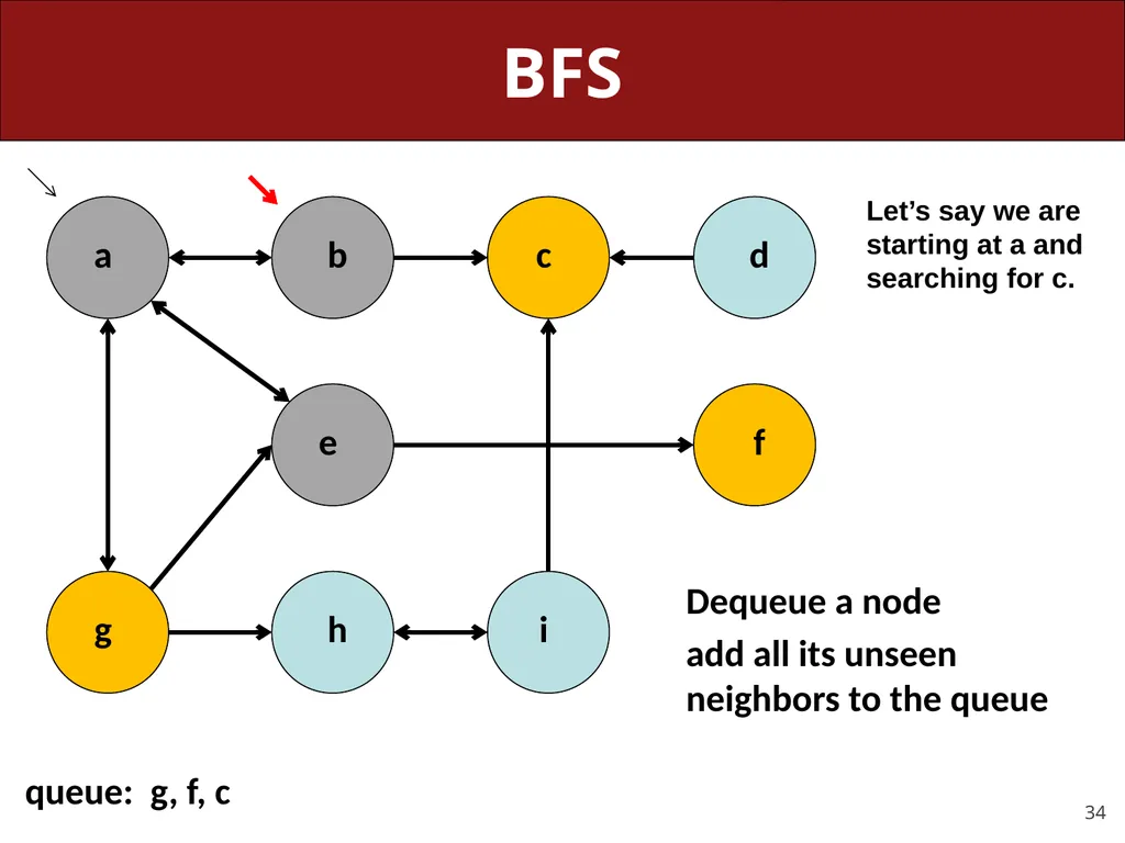
slide34. BFS a b c d f e g h i queue: g, f, c Dequeue a node
add all its unseen neighbors to the queue Let’s say we are starting at a and searching for c.<br>
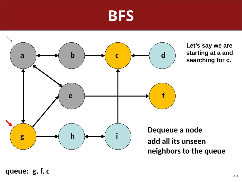
slide35. BFS a b c d f e g h i queue: g, f, c Dequeue a node
add all its unseen neighbors to the queue Let’s say we are starting at a and searching for c.<br>
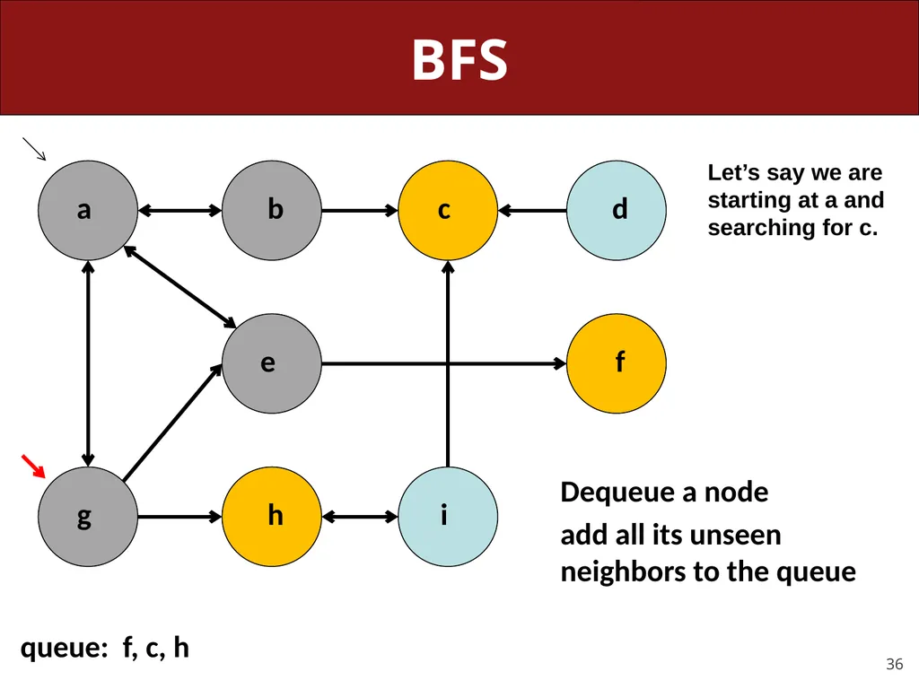
slide36. BFS a b c d f e g h i queue: f, c, h Dequeue a node
add all its unseen neighbors to the queue Let’s say we are starting at a and searching for c.<br>
slide37. BFS a b c d f e g h i queue: f, c, h Dequeue a node
add all its unseen neighbors to the queue Let’s say we are starting at a and searching for c.<br>
slide38. BFS a b c d f e g h i queue: c, h Dequeue a node
add all its unseen neighbors to the queue Let’s say we are starting at a and searching for c.<br>
slide39. BFS a b c d f e g h i queue: c, h Dequeue a node
add all its unseen neighbors to the queue Let’s say we are starting at a and searching for c.<br>
slide40. BFS a b c d f e g h i queue: h Dequeue a node
add all its unseen neighbors to the queue Let’s say we are starting at a and searching for c.<br>
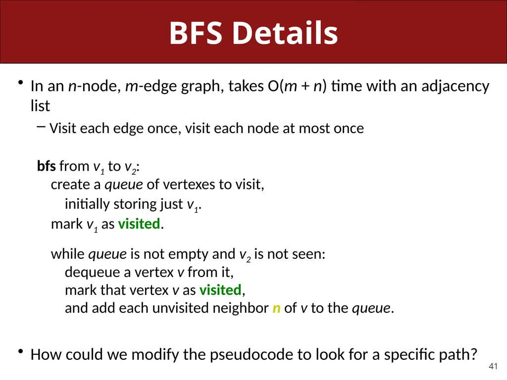
slide41. BFS Details In an n-node, m-edge graph, takes O(m + n) time with an adjacency list
Visit each edge once, visit each node at most once
bfs from v1 to v2:
create a queue of vertexes to visit,
initially storing just v1.
mark v1 as visited.
while queue is not empty and v2 is not seen:
dequeue a vertex v from it,
mark that vertex v as visited,
and add each unvisited neighbor n of v to the queue.
How could we modify the pseudocode to look for a specific path?<br>
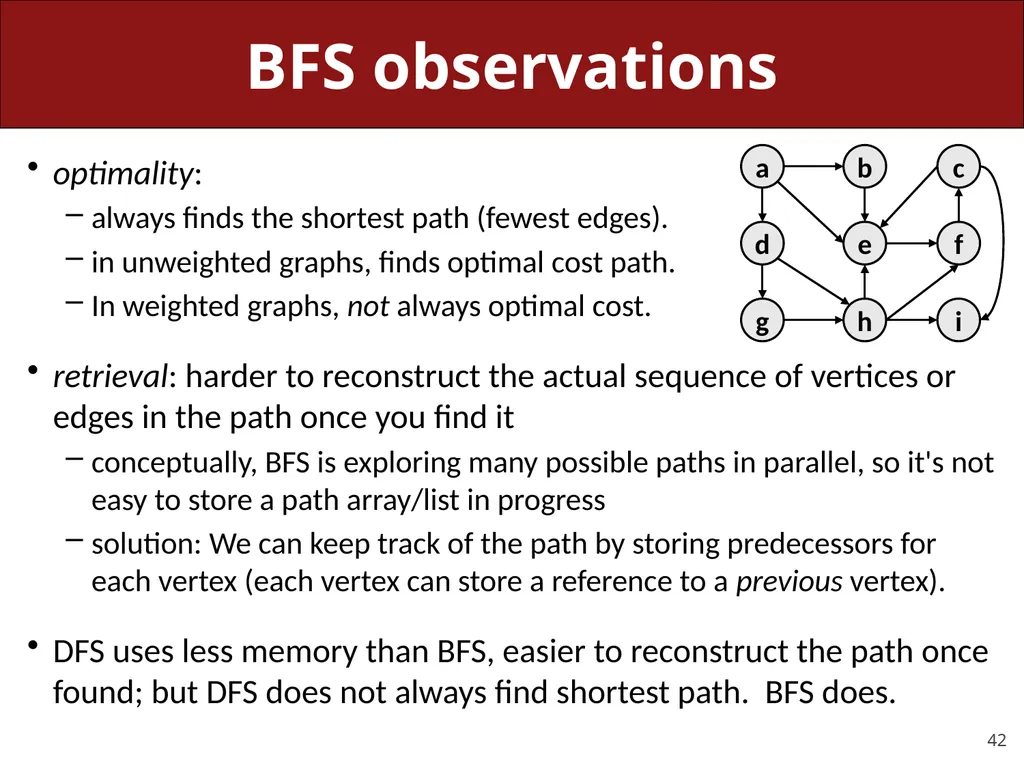
slide42. BFS observations optimality:
always finds the shortest path (fewest edges).
in unweighted graphs, finds optimal cost path.
In weighted graphs, not always optimal cost.
retrieval: harder to reconstruct the actual sequence of vertices or edges in the path once you find it
conceptually, BFS is exploring many possible paths in parallel, so it's not easy to store a path array/list in progress
solution: We can keep track of the path by storing predecessors for each vertex (each vertex can store a reference to a previous vertex).
DFS uses less memory than BFS, easier to reconstruct the path once found; but DFS does not always find shortest path. BFS does.<br>
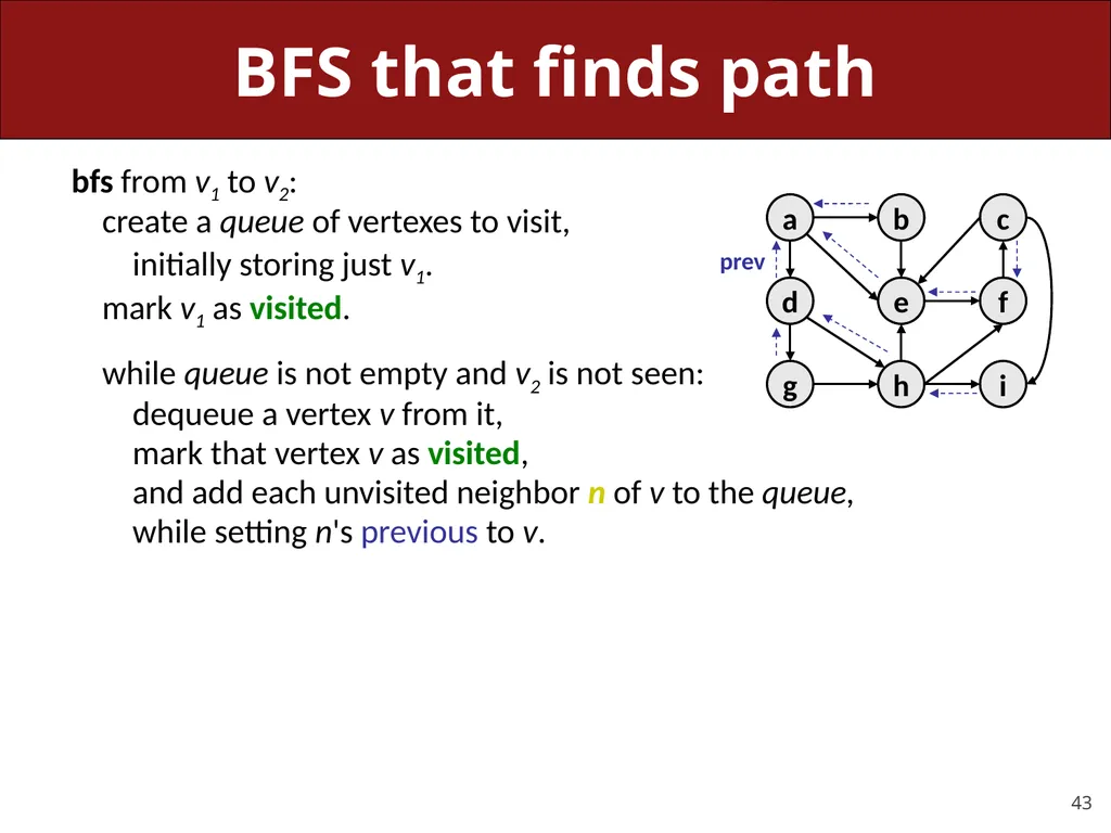
slide43. BFS that finds path bfs from v1 to v2:
create a queue of vertexes to visit,
initially storing just v1.
mark v1 as visited.
while queue is not empty and v2 is not seen:
dequeue a vertex v from it,
mark that vertex v as visited,
and add each unvisited neighbor n of v to the queue,
while setting n's previous to v. prev<br>
slide44. Plan For Today Recap: DFS and BFS
Dijkstra’s Algorithm
Announcements
A* Search<br>
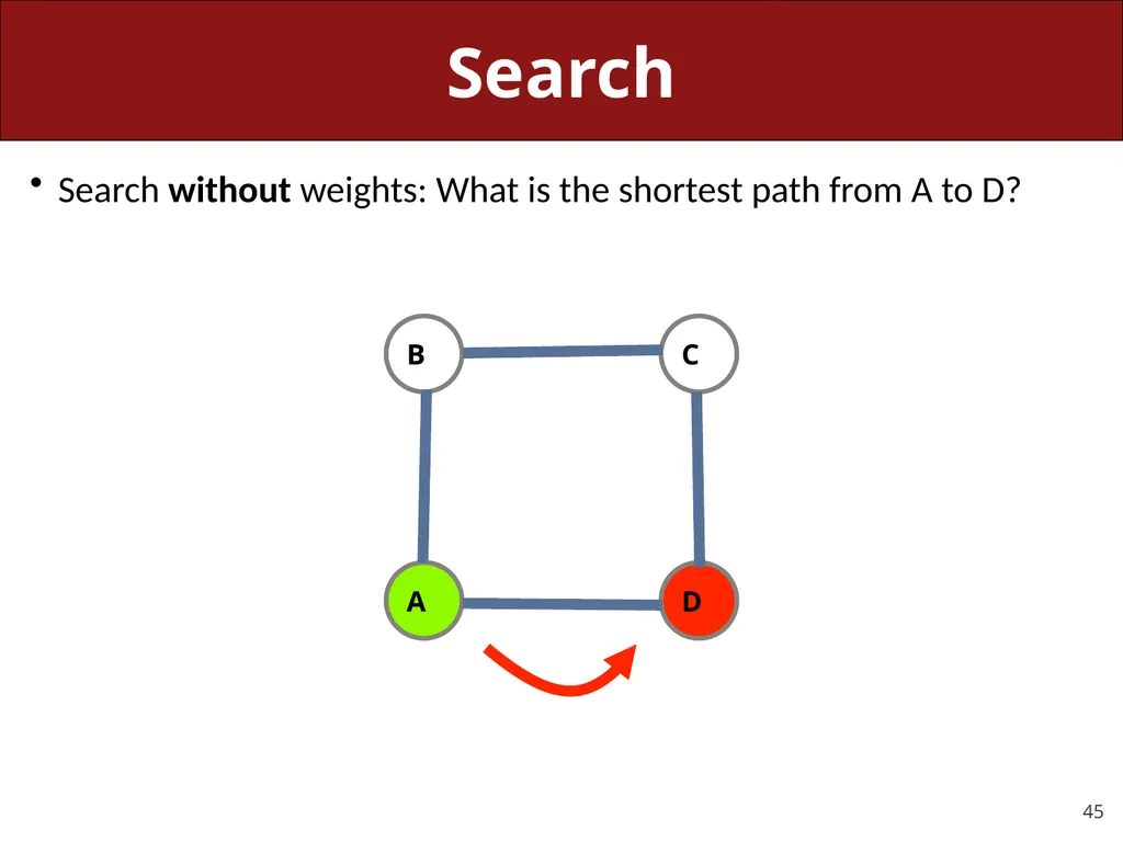
slide45. Search Search without weights: What is the shortest path from A to D?<br>
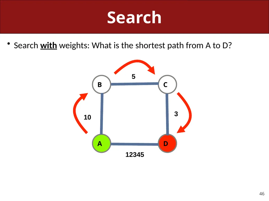
slide46. Search Search with weights: What is the shortest path from A to D? 12345 10 5 3<br>
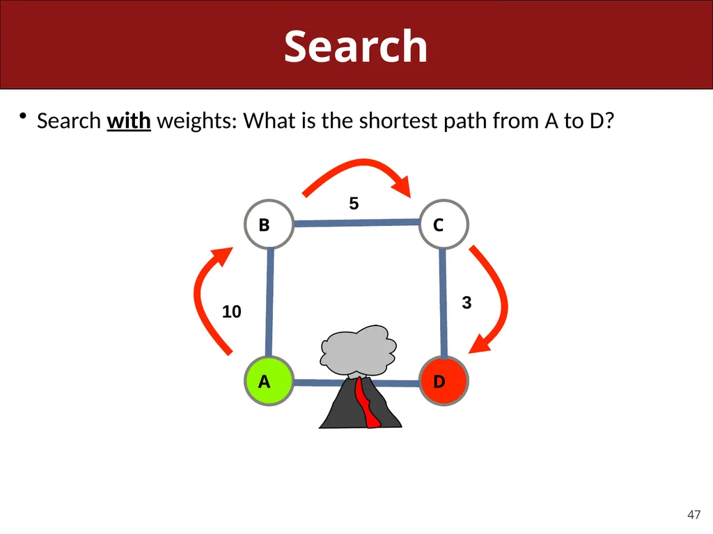
slide47. Search Search with weights: What is the shortest path from A to D? 12345 10 5 3<br>
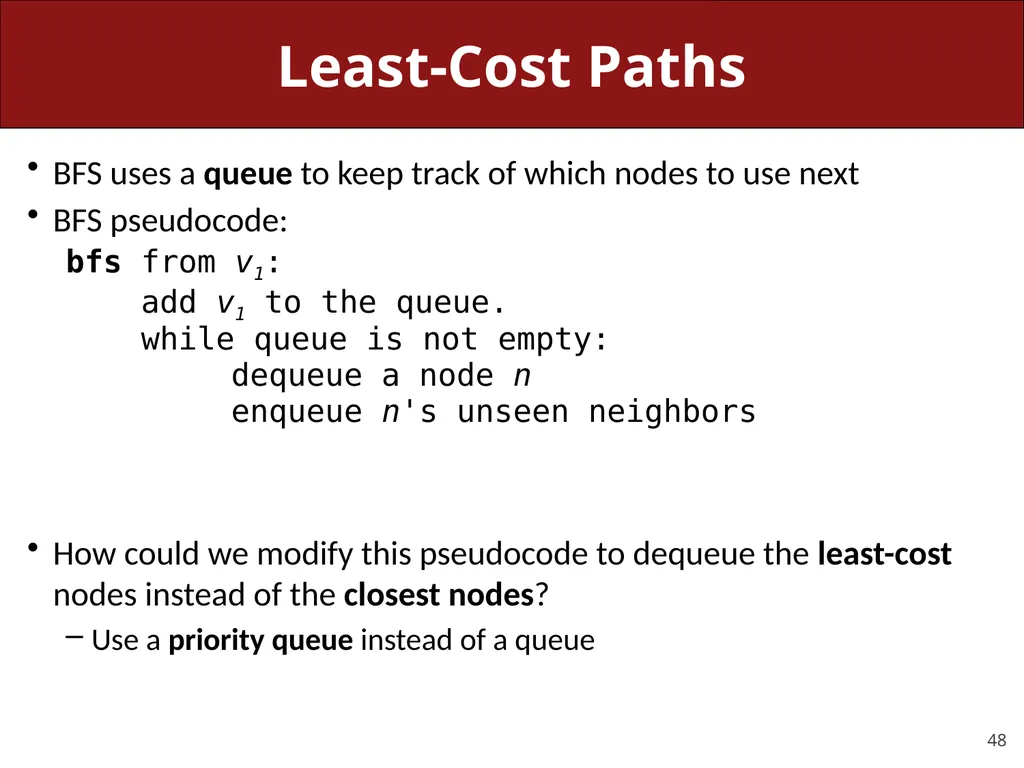
slide48. Least-Cost Paths BFS uses a queue to keep track of which nodes to use next
BFS pseudocode:
bfs from v1:
add v1 to the queue.
while queue is not empty:
dequeue a node n
enqueue n's unseen neighbors
How could we modify this pseudocode to dequeue the least-cost nodes instead of the closest nodes?
Use a priority queue instead of a queue<br>
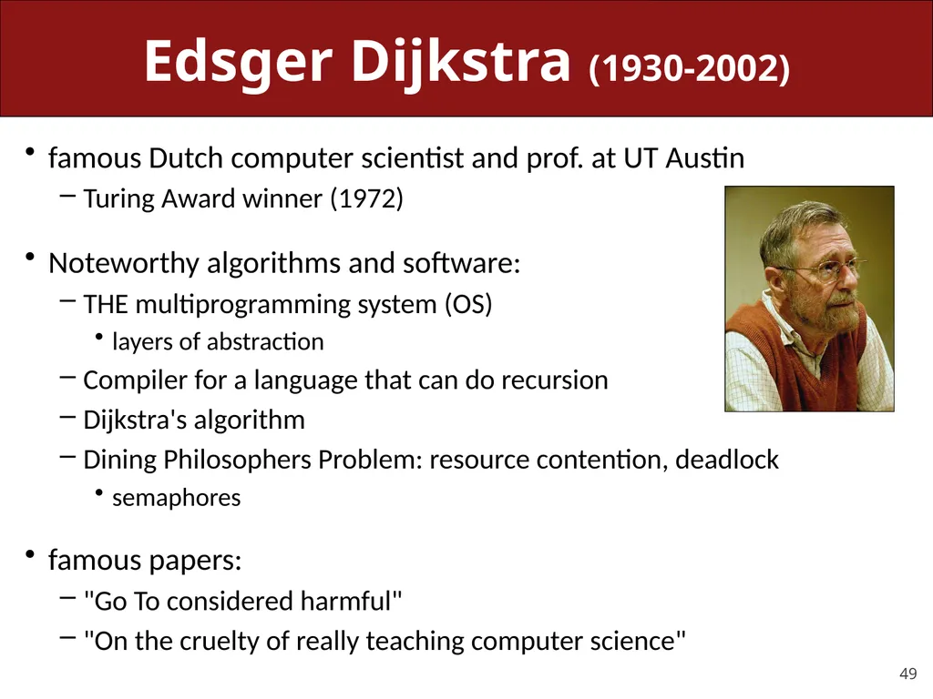
slide49. Edsger Dijkstra (1930-2002) famous Dutch computer scientist and prof. at UT Austin
Turing Award winner (1972)
Noteworthy algorithms and software:
THE multiprogramming system (OS)
layers of abstraction
Compiler for a language that can do recursion
Dijkstra's algorithm
Dining Philosophers Problem: resource contention, deadlock
semaphores
famous papers:
"Go To considered harmful"
"On the cruelty of really teaching computer science"<br>
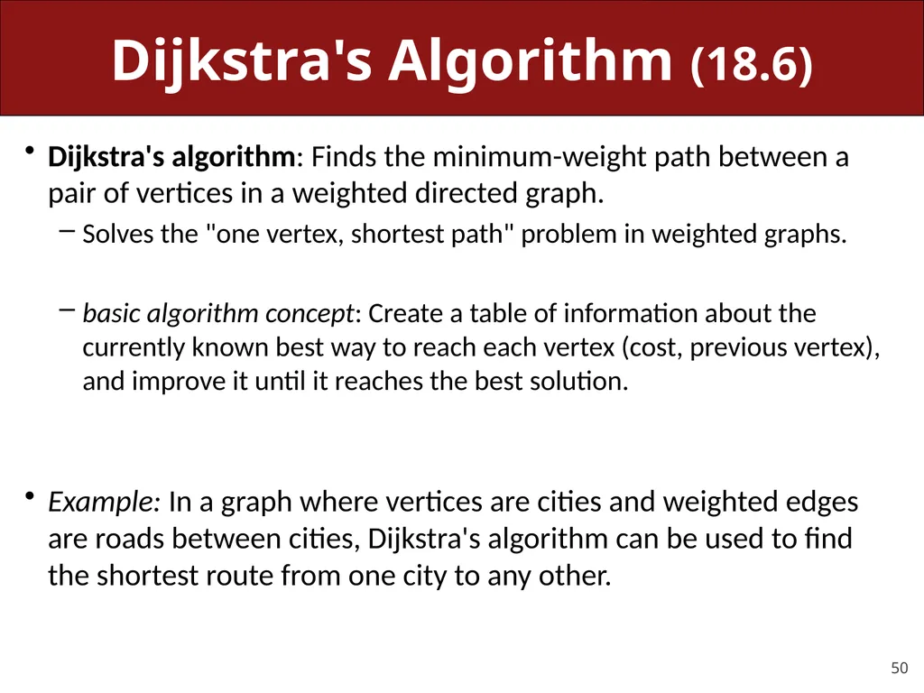
slide50. Dijkstra's Algorithm (18.6) Dijkstra's algorithm: Finds the minimum-weight path between a pair of vertices in a weighted directed graph.
Solves the "one vertex, shortest path" problem in weighted graphs.
basic algorithm concept: Create a table of information about the currently known best way to reach each vertex (cost, previous vertex), and improve it until it reaches the best solution.
Example: In a graph where vertices are cities and weighted edges are roads between cities, Dijkstra's algorithm can be used to find the shortest route from one city to any other.<br>
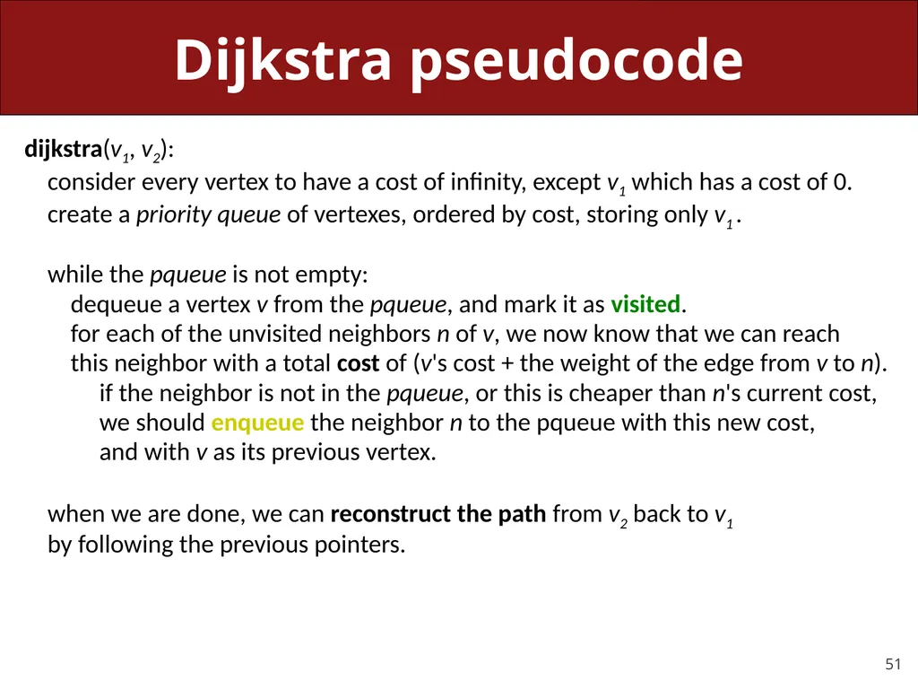
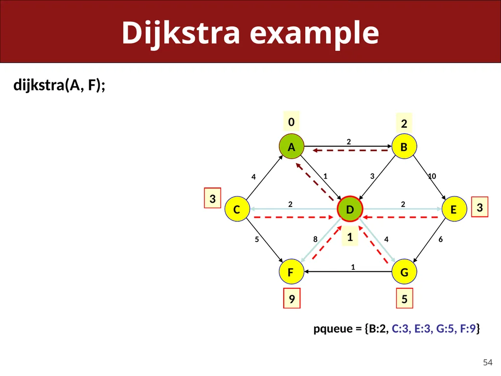
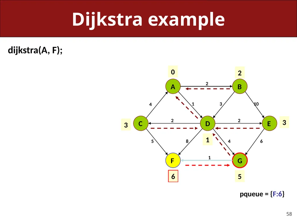
slide51. Dijkstra pseudocode dijkstra(v1, v2):
consider every vertex to have a cost of infinity, except v1 which has a cost of 0.
create a priority queue of vertexes, ordered by cost, storing only v1 .
while the pqueue is not empty:
dequeue a vertex v from the pqueue, and mark it as visited.
for each of the unvisited neighbors n of v, we now know that we can reach
this neighbor with a total cost of (v's cost + the weight of the edge from v to n).
if the neighbor is not in the pqueue, or this is cheaper than n's current cost,
we should enqueue the neighbor n to the pqueue with this new cost,
and with v as its previous vertex.
when we are done, we can reconstruct the path from v2 back to v1
by following the previous pointers.<br>
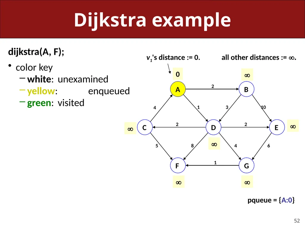
slide52. Dijkstra example dijkstra(A, F);
color key
white: unexamined
yellow: enqueued
green: visited A G F B E C D 4 1 2 10 3 6 4 2 2 8 5 1 0 v1's distance := 0. all other distances := . pqueue = {A:0}<br>
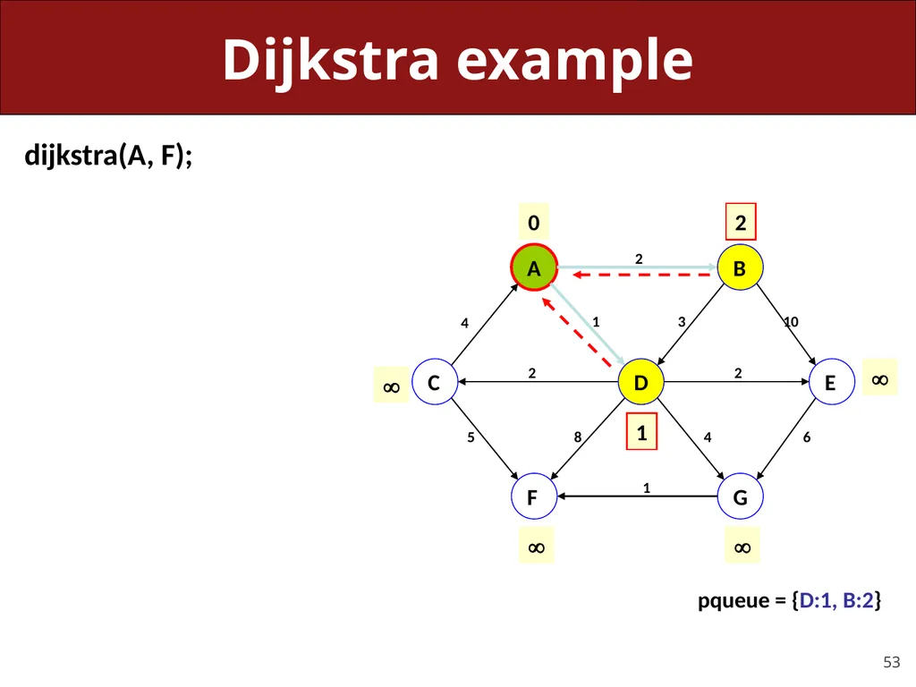
slide53. Dijkstra example dijkstra(A, F); A G F B E C D 4 1 2 10 3 6 4 2 2 8 5 1 0 2 1 pqueue = {D:1, B:2}<br>
slide54. Dijkstra example dijkstra(A, F); pqueue = {B:2, C:3, E:3, G:5, F:9} A G F B E C D 4 1 2 10 3 6 4 2 2 8 5 1 0 2 3 3 1 9 5<br>
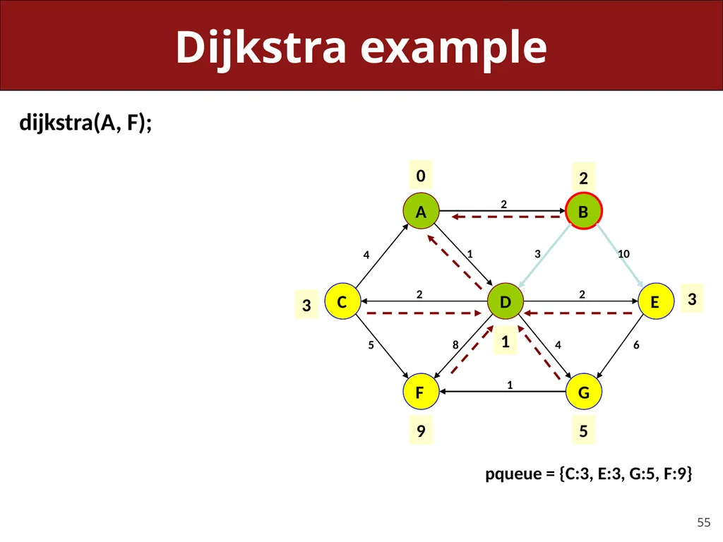
slide55. Dijkstra example dijkstra(A, F); pqueue = {C:3, E:3, G:5, F:9} A G F B E C D 4 1 2 10 3 6 4 2 2 8 5 1 0 2 3 3 1 9 5<br>
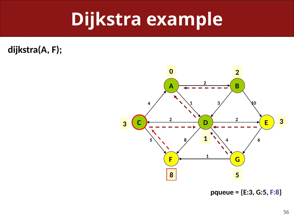
slide56. Dijkstra example dijkstra(A, F); pqueue = {E:3, G:5, F:8} A G F B E C D 4 1 2 10 3 6 4 2 2 8 5 1 0 2 3 3 1 8 5<br>
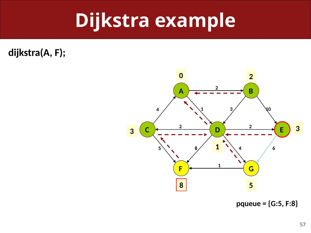
slide57. Dijkstra example dijkstra(A, F); pqueue = {G:5, F:8} A G F B E C D 4 1 2 10 3 6 4 2 2 8 5 1 0 2 3 3 1 8 5<br>
slide58. Dijkstra example dijkstra(A, F); pqueue = {F:6} A G F B E C D 4 1 2 10 3 6 4 2 2 8 5 1 0 2 3 3 1 6 5<br>
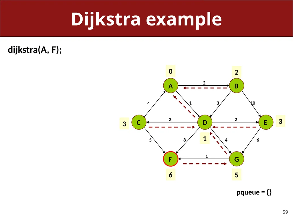
slide59. Dijkstra example dijkstra(A, F); pqueue = {} A G F B E C D 4 1 2 10 3 6 4 2 2 8 5 1 0 2 3 3 1 6 5<br>
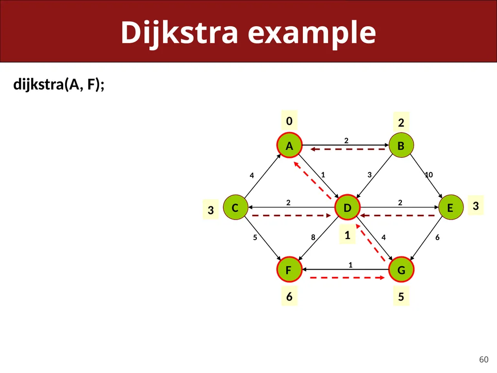
slide60. Dijkstra example dijkstra(A, F); A G F B E C D 4 1 2 10 3 6 4 2 2 8 5 1 0 2 3 3 1 6 5<br>
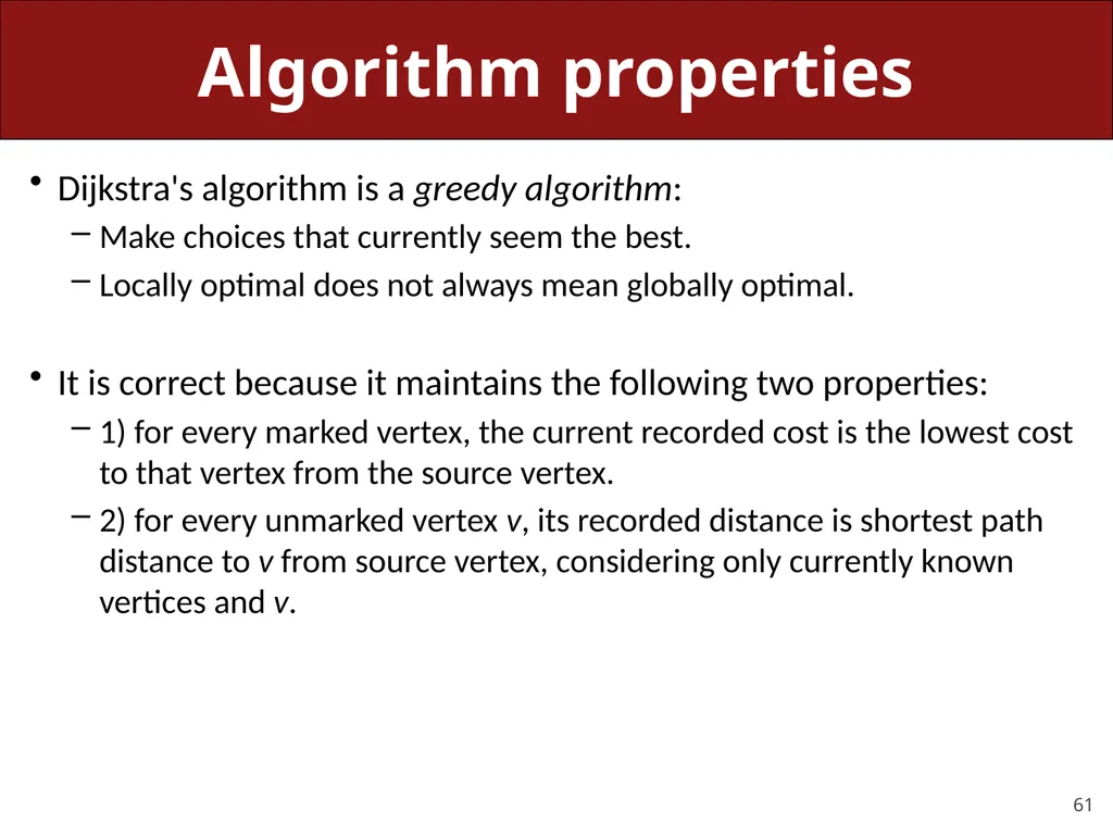
slide61. Algorithm properties Dijkstra's algorithm is a greedy algorithm:
Make choices that currently seem the best.
Locally optimal does not always mean globally optimal.
It is correct because it maintains the following two properties:
1) for every marked vertex, the current recorded cost is the lowest cost to that vertex from the source vertex.
2) for every unmarked vertex v, its recorded distance is shortest path distance to v from source vertex, considering only currently known vertices and v.<br>
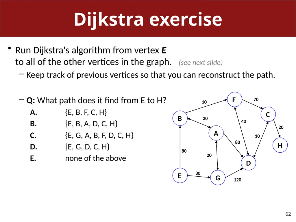
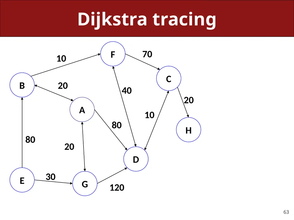
slide62. Dijkstra exercise Run Dijkstra's algorithm from vertex E to all of the other vertices in the graph. (see next slide)
Keep track of previous vertices so that you can reconstruct the path.
Q: What path does it find from E to H?
A. {E, B, F, C, H}
B. {E, B, A, D, C, H}
C. {E, G, A, B, F, D, C, H}
D. {E, G, D, C, H}
E. none of the above<br>
slide63. Dijkstra tracing<br>
slide64. Plan For Today Recap: DFS and BFS
Dijkstra’s Algorithm
Announcements
A* Search<br>
slide65. Announcements Mid-quarter grade reports are available on the course website<br>
slide66. Plan For Today Recap: DFS and BFS
Dijkstra’s Algorithm
Announcements
A* Search<br>
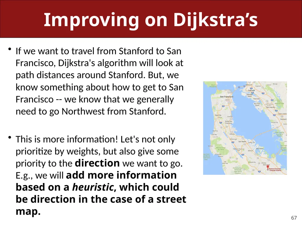
slide67. Improving on Dijkstra’s If we want to travel from Stanford to San Francisco, Dijkstra's algorithm will look at path distances around Stanford. But, we know something about how to get to San Francisco -- we know that we generally need to go Northwest from Stanford.
This is more information! Let's not only prioritize by weights, but also give some priority to the direction we want to go. E.g., we will add more information based on a heuristic, which could be direction in the case of a street map.<br>
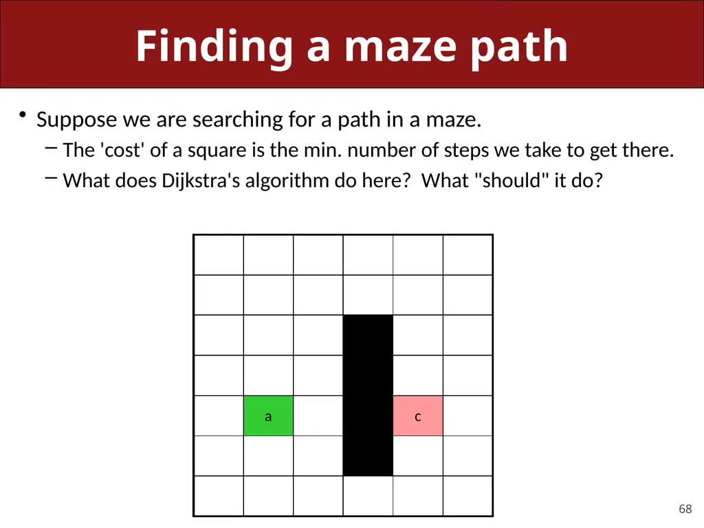
slide68. Finding a maze path Suppose we are searching for a path in a maze.
The 'cost' of a square is the min. number of steps we take to get there.
What does Dijkstra's algorithm do here? What "should" it do?<br>
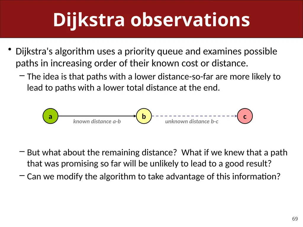
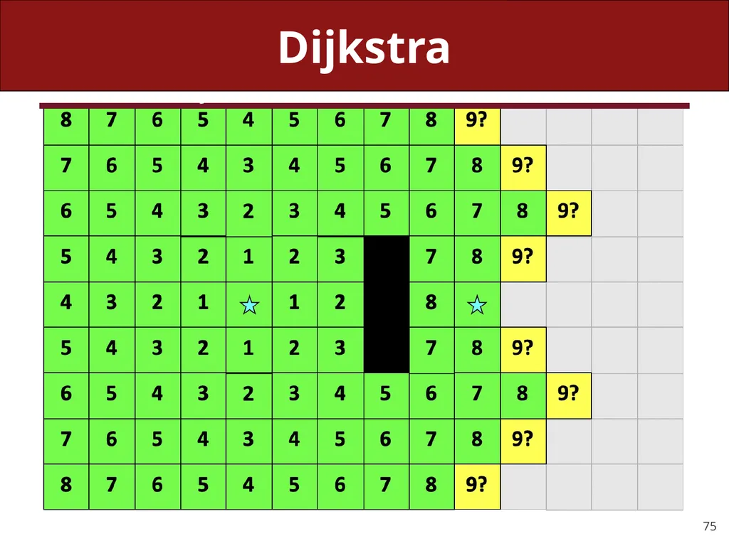
slide69. Dijkstra observations Dijkstra's algorithm uses a priority queue and examines possible paths in increasing order of their known cost or distance.
The idea is that paths with a lower distance-so-far are more likely to lead to paths with a lower total distance at the end.
But what about the remaining distance? What if we knew that a path that was promising so far will be unlikely to lead to a good result?
Can we modify the algorithm to take advantage of this information? a b c known distance a-b unknown distance b-c<br>
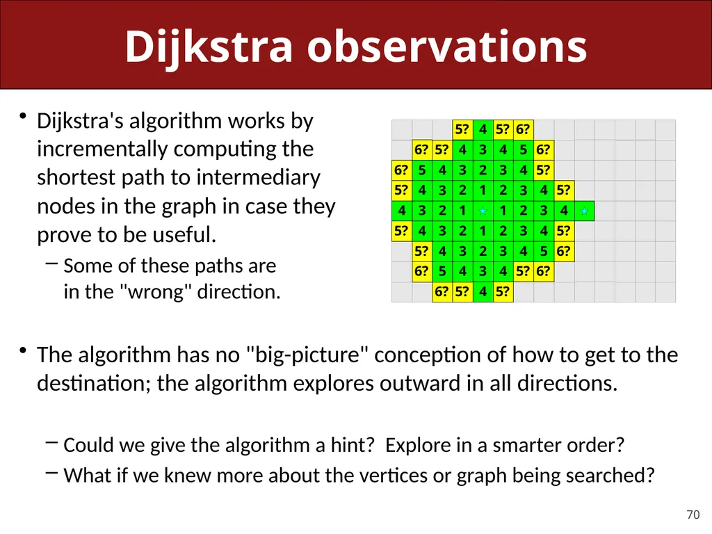
slide70. Dijkstra observations Dijkstra's algorithm works by incrementally computing the shortest path to intermediary nodes in the graph in case they prove to be useful.
Some of these paths are in the "wrong" direction.
The algorithm has no "big-picture" conception of how to get to the destination; the algorithm explores outward in all directions.
Could we give the algorithm a hint? Explore in a smarter order?
What if we knew more about the vertices or graph being searched?<br>
slide71. Heuristics heuristic: A speculation, estimation, or educated guess that guides the search for a solution to a problem.
Example: Spam filters flag a message as probable spam if it contains certain words, has certain attachments, is sent to many people, ...
In the context of graph searches: A function that approximates the distance from a known vertex to another destination vertex.
Example: Estimate the distance between two places on a Google Maps graph to be the direct straight-line distance between them.
admissible heuristic: One that never overestimates the distance.
Okay if the heuristic underestimates sometimes (e.g. Google Maps).
Only ignore paths that in the best case are worse than your current path<br>
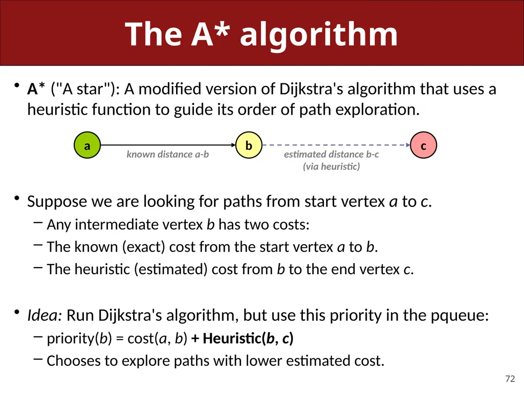
slide72. The A* algorithm A* ("A star"): A modified version of Dijkstra's algorithm that uses a heuristic function to guide its order of path exploration.
Suppose we are looking for paths from start vertex a to c.
Any intermediate vertex b has two costs:
The known (exact) cost from the start vertex a to b.
The heuristic (estimated) cost from b to the end vertex c.
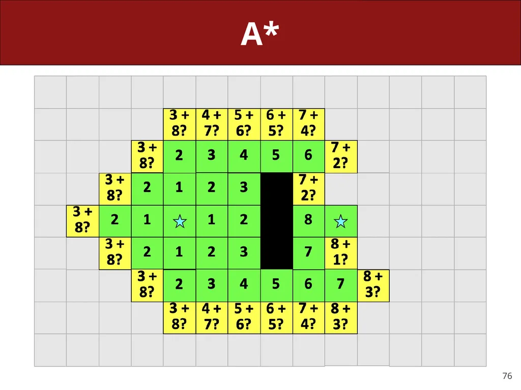
Idea: Run Dijkstra's algorithm, but use this priority in the pqueue:
priority(b) = cost(a, b) + Heuristic(b, c)
Chooses to explore paths with lower estimated cost. a b c known distance a-b estimated distance b-c (via heuristic)<br>
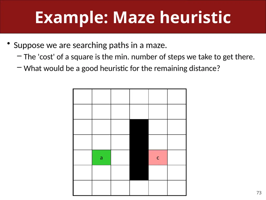
slide73. Example: Maze heuristic Suppose we are searching paths in a maze.
The 'cost' of a square is the min. number of steps we take to get there.
What would be a good heuristic for the remaining distance?<br>
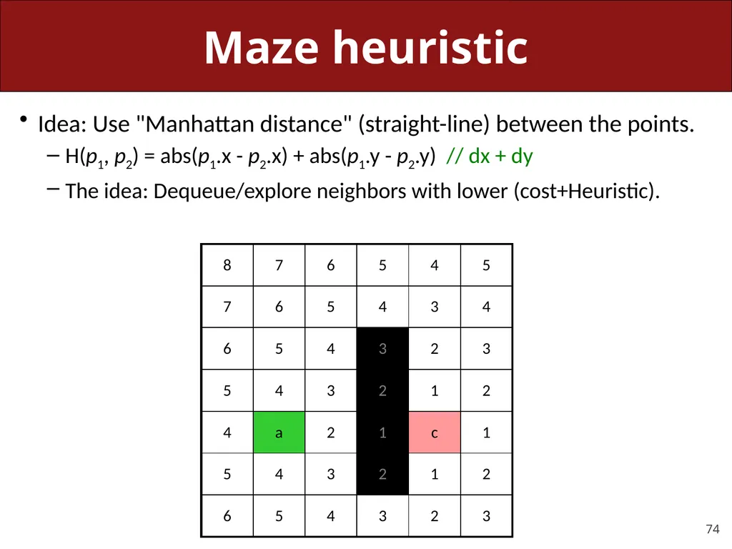
slide74. Maze heuristic Idea: Use "Manhattan distance" (straight-line) between the points.
H(p1, p2) = abs(p1.x - p2.x) + abs(p1.y - p2.y) // dx + dy
The idea: Dequeue/explore neighbors with lower (cost+Heuristic).<br>
slide75. Dijkstra<br>
slide76. A*<br>
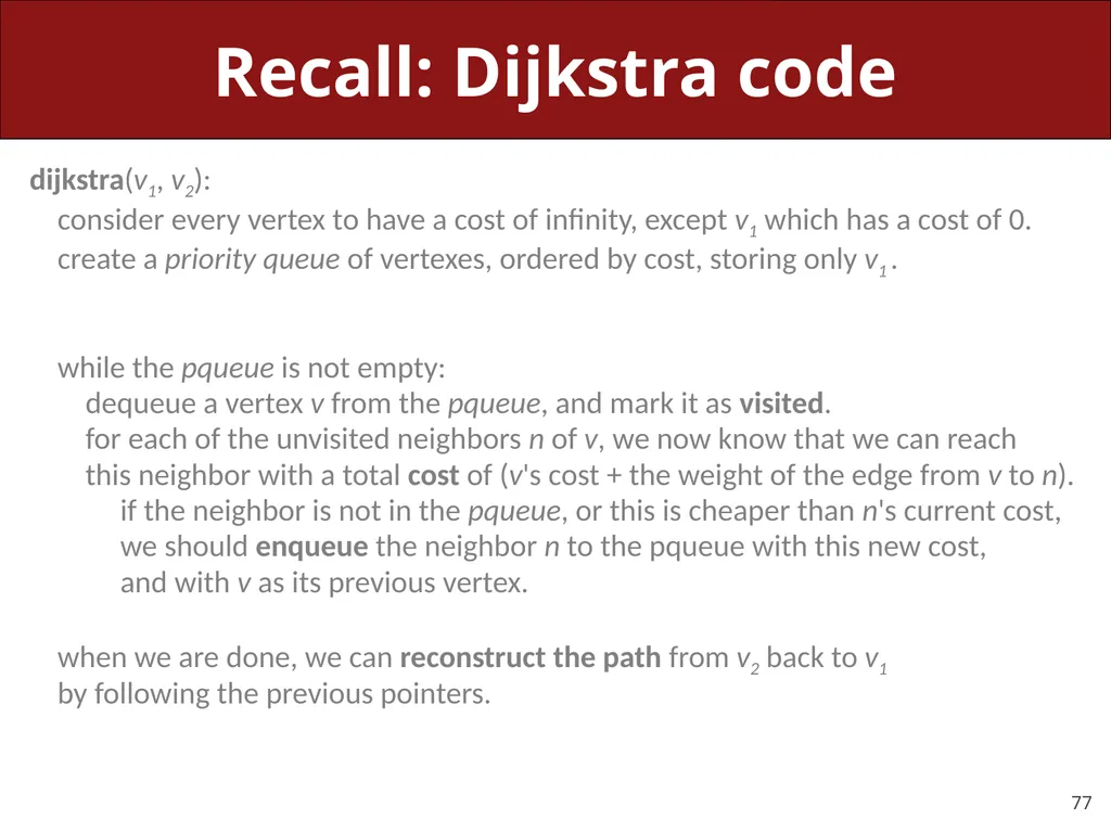
slide77. Recall: Dijkstra code dijkstra(v1, v2):
consider every vertex to have a cost of infinity, except v1 which has a cost of 0.
create a priority queue of vertexes, ordered by cost, storing only v1 .
while the pqueue is not empty:
dequeue a vertex v from the pqueue, and mark it as visited.
for each of the unvisited neighbors n of v, we now know that we can reach
this neighbor with a total cost of (v's cost + the weight of the edge from v to n).
if the neighbor is not in the pqueue, or this is cheaper than n's current cost,
we should enqueue the neighbor n to the pqueue with this new cost,
and with v as its previous vertex.
when we are done, we can reconstruct the path from v2 back to v1
by following the previous pointers.<br>
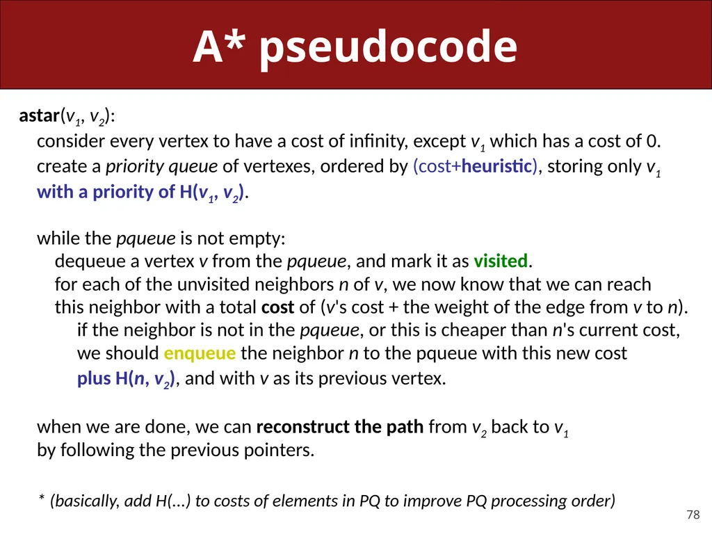
slide78. A* pseudocode astar(v1, v2):
consider every vertex to have a cost of infinity, except v1 which has a cost of 0.
create a priority queue of vertexes, ordered by (cost+heuristic), storing only v1
with a priority of H(v1, v2).
while the pqueue is not empty:
dequeue a vertex v from the pqueue, and mark it as visited.
for each of the unvisited neighbors n of v, we now know that we can reach
this neighbor with a total cost of (v's cost + the weight of the edge from v to n).
if the neighbor is not in the pqueue, or this is cheaper than n's current cost,
we should enqueue the neighbor n to the pqueue with this new cost
plus H(n, v2), and with v as its previous vertex.
when we are done, we can reconstruct the path from v2 back to v1
by following the previous pointers.
* (basically, add H(...) to costs of elements in PQ to improve PQ processing order)<br>
slide79. Recap Recap: DFS and BFS
Dijkstra’s Algorithm
Announcements
A* Search
Next time: Minimum Spanning Trees<br>
Programming Abstractions in C++, Chapter 18<br>
slide2. Plan For Today Recap: DFS and BFS
Dijkstra’s Algorithm
Announcements
A* Search<br>
slide3. Plan For Today Recap: DFS and BFS
Dijkstra’s Algorithm
Announcements
A* Search<br>
slide4. Depth-first search (18.4) depth-first search (DFS): Finds a path between two vertices by exploring each possible path as far as possible before backtracking.
Often implemented recursively.
Many graph algorithms involve visiting or marking vertices.
DFS from a to h (assuming A-Z order) visits:
a
b
e
f
c
i
d
g
h
path found: {a, d, g, h}<br>
slide5. DFS Mark current as visited
Explore all the unvisited nodes from this node A B C D F E I H G Let’s say we are starting at A and searching for C.<br>
slide6. DFS Mark current as visited
Explore all the unvisited nodes from this node A B C D F E I H G Let’s say we are starting at A and searching for C.<br>
slide7. DFS Mark current as visited
Explore all the unvisited nodes from this node A B C D F E I H G Let’s say we are starting at A and searching for C.<br>
slide8. DFS Mark current as visited
Explore all the unvisited nodes from this node A B C D F E I H G Let’s say we are starting at A and searching for C.<br>
slide9. DFS Mark current as visited
Explore all the unvisited nodes from this node A B C D F E I H G Let’s say we are starting at A and searching for C.<br>
slide10. DFS Mark current as visited
Explore all the unvisited nodes from this node A B C D F E I H G Let’s say we are starting at A and searching for C.<br>
slide11. DFS Mark current as visited
Explore all the unvisited nodes from this node A B C D F E I H G Let’s say we are starting at A and searching for C.<br>
slide12. DFS Mark current as visited
Explore all the unvisited nodes from this node A B C D F E I H G Let’s say we are starting at A and searching for C.<br>
slide13. DFS Mark current as visited
Explore all the unvisited nodes from this node A B C D F E I H G Let’s say we are starting at A and searching for C.<br>
slide14. DFS Mark current as visited
Explore all the unvisited nodes from this node A B C D F E I H G Let’s say we are starting at A and searching for C.<br>
slide15. DFS Mark current as visited
Explore all the unvisited nodes from this node A B C D F E I H G Let’s say we are starting at A and searching for C.<br>
slide16. DFS Mark current as visited
Explore all the unvisited nodes from this node A B C D F E I H G Let’s say we are starting at A and searching for C.<br>
slide17. DFS Mark current as visited
Explore all the unvisited nodes from this node A B C D F E I H G Let’s say we are starting at A and searching for C.<br>
slide18. DFS Mark current as visited
Explore all the unvisited nodes from this node A B C D F E I H G Let’s say we are starting at A and searching for C.<br>
slide19. DFS Mark current as visited
Explore all the unvisited nodes from this node A B C D F E I H G Let’s say we are starting at A and searching for C.<br>
slide20. DFS Mark current as visited
Explore all the unvisited nodes from this node A B C D F E I H G Let’s say we are starting at A and searching for C.<br>
slide21. DFS Mark current as visited
Explore all the unvisited nodes from this node A B C D F E I H G Let’s say we are starting at A and searching for C.<br>
slide22. DFS Mark current as visited
Explore all the unvisited nodes from this node A B C D F E I H G Let’s say we are starting at A and searching for C.<br>
slide23. DFS Mark current as visited
Explore all the unvisited nodes from this node A B C D F E I H G Let’s say we are starting at A and searching for C.<br>
slide24. DFS Details In an n-node, m-edge graph, takes O(m + n) time with an adjacency list
Visit each edge once, visit each node at most once
Pseudocode:
dfs from v1:
mark v1 as seen.
for each of v1's unvisited neighbors n: dfs(n)<br>
slide25. DFS that finds path dfs from v1 to v2:
mark v1 as visited, and add to path.
perform a dfs from each of v1's unvisited neighbors n to v2: if dfs(n, v2) succeeds: a path is found! yay!
if all neighbors fail: remove v1 from path.
To retrieve the DFS path found, pass a collection parameter to each call and choose-explore-unchoose.<br>
slide26. DFS observations discovery: DFS is guaranteed to find a path if one exists.
retrieval: It is easy to retrieve exactly what the path is (the sequence of edges taken) if we find it
choose - explore - unchoose
optimality: not optimal. DFS is guaranteed to find a path, not necessarily the best/shortest path
Example: dfs(a, i) returns {a, b, e, f, c, i} rather than {a, d, h, i}.<br>
slide27. Finding Shortest Paths We can find paths between two nodes, but how can we find the shortest path?
Fewest number of steps to complete a task?
Least amount of edits between two words?<br>
slide28. Breadth-First Search (BFS) Idea: processing a node involves knowing we need to visit all its neighbors (just like DFS)
Need to keep a TODO list of nodes to process
Keep a Queue of nodes as our TODO list
Idea: dequeue a node, enqueue all its neighbors
Still will return the same nodes as reachable, just might have shorter paths<br>
slide29. BFS a b c d f e g h i queue: a Dequeue a node
add all its unseen neighbors to the queue Let’s say we are starting at a and searching for c.<br>
slide30. BFS a b c d f e g h i queue: e, b, g Dequeue a node
add all its unseen neighbors to the queue Let’s say we are starting at a and searching for c.<br>
slide31. BFS a b c d f e g h i queue: e, b, g Dequeue a node
add all its unseen neighbors to the queue Let’s say we are starting at a and searching for c.<br>
slide32. BFS a b c d f e g h i queue: b, g, f Dequeue a node
add all its unseen neighbors to the queue Let’s say we are starting at a and searching for c.<br>
slide33. BFS a b c d f e g h i queue: b, g, f Dequeue a node
add all its unseen neighbors to the queue Let’s say we are starting at a and searching for c.<br>
slide34. BFS a b c d f e g h i queue: g, f, c Dequeue a node
add all its unseen neighbors to the queue Let’s say we are starting at a and searching for c.<br>
slide35. BFS a b c d f e g h i queue: g, f, c Dequeue a node
add all its unseen neighbors to the queue Let’s say we are starting at a and searching for c.<br>
slide36. BFS a b c d f e g h i queue: f, c, h Dequeue a node
add all its unseen neighbors to the queue Let’s say we are starting at a and searching for c.<br>
slide37. BFS a b c d f e g h i queue: f, c, h Dequeue a node
add all its unseen neighbors to the queue Let’s say we are starting at a and searching for c.<br>
slide38. BFS a b c d f e g h i queue: c, h Dequeue a node
add all its unseen neighbors to the queue Let’s say we are starting at a and searching for c.<br>
slide39. BFS a b c d f e g h i queue: c, h Dequeue a node
add all its unseen neighbors to the queue Let’s say we are starting at a and searching for c.<br>
slide40. BFS a b c d f e g h i queue: h Dequeue a node
add all its unseen neighbors to the queue Let’s say we are starting at a and searching for c.<br>
slide41. BFS Details In an n-node, m-edge graph, takes O(m + n) time with an adjacency list
Visit each edge once, visit each node at most once
bfs from v1 to v2:
create a queue of vertexes to visit,
initially storing just v1.
mark v1 as visited.
while queue is not empty and v2 is not seen:
dequeue a vertex v from it,
mark that vertex v as visited,
and add each unvisited neighbor n of v to the queue.
How could we modify the pseudocode to look for a specific path?<br>
slide42. BFS observations optimality:
always finds the shortest path (fewest edges).
in unweighted graphs, finds optimal cost path.
In weighted graphs, not always optimal cost.
retrieval: harder to reconstruct the actual sequence of vertices or edges in the path once you find it
conceptually, BFS is exploring many possible paths in parallel, so it's not easy to store a path array/list in progress
solution: We can keep track of the path by storing predecessors for each vertex (each vertex can store a reference to a previous vertex).
DFS uses less memory than BFS, easier to reconstruct the path once found; but DFS does not always find shortest path. BFS does.<br>
slide43. BFS that finds path bfs from v1 to v2:
create a queue of vertexes to visit,
initially storing just v1.
mark v1 as visited.
while queue is not empty and v2 is not seen:
dequeue a vertex v from it,
mark that vertex v as visited,
and add each unvisited neighbor n of v to the queue,
while setting n's previous to v. prev<br>
slide44. Plan For Today Recap: DFS and BFS
Dijkstra’s Algorithm
Announcements
A* Search<br>
slide45. Search Search without weights: What is the shortest path from A to D?<br>
slide46. Search Search with weights: What is the shortest path from A to D? 12345 10 5 3<br>
slide47. Search Search with weights: What is the shortest path from A to D? 12345 10 5 3<br>
slide48. Least-Cost Paths BFS uses a queue to keep track of which nodes to use next
BFS pseudocode:
bfs from v1:
add v1 to the queue.
while queue is not empty:
dequeue a node n
enqueue n's unseen neighbors
How could we modify this pseudocode to dequeue the least-cost nodes instead of the closest nodes?
Use a priority queue instead of a queue<br>
slide49. Edsger Dijkstra (1930-2002) famous Dutch computer scientist and prof. at UT Austin
Turing Award winner (1972)
Noteworthy algorithms and software:
THE multiprogramming system (OS)
layers of abstraction
Compiler for a language that can do recursion
Dijkstra's algorithm
Dining Philosophers Problem: resource contention, deadlock
semaphores
famous papers:
"Go To considered harmful"
"On the cruelty of really teaching computer science"<br>
slide50. Dijkstra's Algorithm (18.6) Dijkstra's algorithm: Finds the minimum-weight path between a pair of vertices in a weighted directed graph.
Solves the "one vertex, shortest path" problem in weighted graphs.
basic algorithm concept: Create a table of information about the currently known best way to reach each vertex (cost, previous vertex), and improve it until it reaches the best solution.
Example: In a graph where vertices are cities and weighted edges are roads between cities, Dijkstra's algorithm can be used to find the shortest route from one city to any other.<br>
slide51. Dijkstra pseudocode dijkstra(v1, v2):
consider every vertex to have a cost of infinity, except v1 which has a cost of 0.
create a priority queue of vertexes, ordered by cost, storing only v1 .
while the pqueue is not empty:
dequeue a vertex v from the pqueue, and mark it as visited.
for each of the unvisited neighbors n of v, we now know that we can reach
this neighbor with a total cost of (v's cost + the weight of the edge from v to n).
if the neighbor is not in the pqueue, or this is cheaper than n's current cost,
we should enqueue the neighbor n to the pqueue with this new cost,
and with v as its previous vertex.
when we are done, we can reconstruct the path from v2 back to v1
by following the previous pointers.<br>
slide52. Dijkstra example dijkstra(A, F);
color key
white: unexamined
yellow: enqueued
green: visited A G F B E C D 4 1 2 10 3 6 4 2 2 8 5 1 0 v1's distance := 0. all other distances := . pqueue = {A:0}<br>
slide53. Dijkstra example dijkstra(A, F); A G F B E C D 4 1 2 10 3 6 4 2 2 8 5 1 0 2 1 pqueue = {D:1, B:2}<br>
slide54. Dijkstra example dijkstra(A, F); pqueue = {B:2, C:3, E:3, G:5, F:9} A G F B E C D 4 1 2 10 3 6 4 2 2 8 5 1 0 2 3 3 1 9 5<br>
slide55. Dijkstra example dijkstra(A, F); pqueue = {C:3, E:3, G:5, F:9} A G F B E C D 4 1 2 10 3 6 4 2 2 8 5 1 0 2 3 3 1 9 5<br>
slide56. Dijkstra example dijkstra(A, F); pqueue = {E:3, G:5, F:8} A G F B E C D 4 1 2 10 3 6 4 2 2 8 5 1 0 2 3 3 1 8 5<br>
slide57. Dijkstra example dijkstra(A, F); pqueue = {G:5, F:8} A G F B E C D 4 1 2 10 3 6 4 2 2 8 5 1 0 2 3 3 1 8 5<br>
slide58. Dijkstra example dijkstra(A, F); pqueue = {F:6} A G F B E C D 4 1 2 10 3 6 4 2 2 8 5 1 0 2 3 3 1 6 5<br>
slide59. Dijkstra example dijkstra(A, F); pqueue = {} A G F B E C D 4 1 2 10 3 6 4 2 2 8 5 1 0 2 3 3 1 6 5<br>
slide60. Dijkstra example dijkstra(A, F); A G F B E C D 4 1 2 10 3 6 4 2 2 8 5 1 0 2 3 3 1 6 5<br>
slide61. Algorithm properties Dijkstra's algorithm is a greedy algorithm:
Make choices that currently seem the best.
Locally optimal does not always mean globally optimal.
It is correct because it maintains the following two properties:
1) for every marked vertex, the current recorded cost is the lowest cost to that vertex from the source vertex.
2) for every unmarked vertex v, its recorded distance is shortest path distance to v from source vertex, considering only currently known vertices and v.<br>
slide62. Dijkstra exercise Run Dijkstra's algorithm from vertex E to all of the other vertices in the graph. (see next slide)
Keep track of previous vertices so that you can reconstruct the path.
Q: What path does it find from E to H?
A. {E, B, F, C, H}
B. {E, B, A, D, C, H}
C. {E, G, A, B, F, D, C, H}
D. {E, G, D, C, H}
E. none of the above<br>
slide63. Dijkstra tracing<br>
slide64. Plan For Today Recap: DFS and BFS
Dijkstra’s Algorithm
Announcements
A* Search<br>
slide65. Announcements Mid-quarter grade reports are available on the course website<br>
slide66. Plan For Today Recap: DFS and BFS
Dijkstra’s Algorithm
Announcements
A* Search<br>
slide67. Improving on Dijkstra’s If we want to travel from Stanford to San Francisco, Dijkstra's algorithm will look at path distances around Stanford. But, we know something about how to get to San Francisco -- we know that we generally need to go Northwest from Stanford.
This is more information! Let's not only prioritize by weights, but also give some priority to the direction we want to go. E.g., we will add more information based on a heuristic, which could be direction in the case of a street map.<br>
slide68. Finding a maze path Suppose we are searching for a path in a maze.
The 'cost' of a square is the min. number of steps we take to get there.
What does Dijkstra's algorithm do here? What "should" it do?<br>
slide69. Dijkstra observations Dijkstra's algorithm uses a priority queue and examines possible paths in increasing order of their known cost or distance.
The idea is that paths with a lower distance-so-far are more likely to lead to paths with a lower total distance at the end.
But what about the remaining distance? What if we knew that a path that was promising so far will be unlikely to lead to a good result?
Can we modify the algorithm to take advantage of this information? a b c known distance a-b unknown distance b-c<br>
slide70. Dijkstra observations Dijkstra's algorithm works by incrementally computing the shortest path to intermediary nodes in the graph in case they prove to be useful.
Some of these paths are in the "wrong" direction.
The algorithm has no "big-picture" conception of how to get to the destination; the algorithm explores outward in all directions.
Could we give the algorithm a hint? Explore in a smarter order?
What if we knew more about the vertices or graph being searched?<br>
slide71. Heuristics heuristic: A speculation, estimation, or educated guess that guides the search for a solution to a problem.
Example: Spam filters flag a message as probable spam if it contains certain words, has certain attachments, is sent to many people, ...
In the context of graph searches: A function that approximates the distance from a known vertex to another destination vertex.
Example: Estimate the distance between two places on a Google Maps graph to be the direct straight-line distance between them.
admissible heuristic: One that never overestimates the distance.
Okay if the heuristic underestimates sometimes (e.g. Google Maps).
Only ignore paths that in the best case are worse than your current path<br>
slide72. The A* algorithm A* ("A star"): A modified version of Dijkstra's algorithm that uses a heuristic function to guide its order of path exploration.
Suppose we are looking for paths from start vertex a to c.
Any intermediate vertex b has two costs:
The known (exact) cost from the start vertex a to b.
The heuristic (estimated) cost from b to the end vertex c.
Idea: Run Dijkstra's algorithm, but use this priority in the pqueue:
priority(b) = cost(a, b) + Heuristic(b, c)
Chooses to explore paths with lower estimated cost. a b c known distance a-b estimated distance b-c (via heuristic)<br>
slide73. Example: Maze heuristic Suppose we are searching paths in a maze.
The 'cost' of a square is the min. number of steps we take to get there.
What would be a good heuristic for the remaining distance?<br>
slide74. Maze heuristic Idea: Use "Manhattan distance" (straight-line) between the points.
H(p1, p2) = abs(p1.x - p2.x) + abs(p1.y - p2.y) // dx + dy
The idea: Dequeue/explore neighbors with lower (cost+Heuristic).<br>
slide75. Dijkstra<br>
slide76. A*<br>
slide77. Recall: Dijkstra code dijkstra(v1, v2):
consider every vertex to have a cost of infinity, except v1 which has a cost of 0.
create a priority queue of vertexes, ordered by cost, storing only v1 .
while the pqueue is not empty:
dequeue a vertex v from the pqueue, and mark it as visited.
for each of the unvisited neighbors n of v, we now know that we can reach
this neighbor with a total cost of (v's cost + the weight of the edge from v to n).
if the neighbor is not in the pqueue, or this is cheaper than n's current cost,
we should enqueue the neighbor n to the pqueue with this new cost,
and with v as its previous vertex.
when we are done, we can reconstruct the path from v2 back to v1
by following the previous pointers.<br>
slide78. A* pseudocode astar(v1, v2):
consider every vertex to have a cost of infinity, except v1 which has a cost of 0.
create a priority queue of vertexes, ordered by (cost+heuristic), storing only v1
with a priority of H(v1, v2).
while the pqueue is not empty:
dequeue a vertex v from the pqueue, and mark it as visited.
for each of the unvisited neighbors n of v, we now know that we can reach
this neighbor with a total cost of (v's cost + the weight of the edge from v to n).
if the neighbor is not in the pqueue, or this is cheaper than n's current cost,
we should enqueue the neighbor n to the pqueue with this new cost
plus H(n, v2), and with v as its previous vertex.
when we are done, we can reconstruct the path from v2 back to v1
by following the previous pointers.
* (basically, add H(...) to costs of elements in PQ to improve PQ processing order)<br>
slide79. Recap Recap: DFS and BFS
Dijkstra’s Algorithm
Announcements
A* Search
Next time: Minimum Spanning Trees<br>