CS 581 Tandy Warnow Today Brief intro to Newick

slide1. CS 581 Tandy Warnow<br>
slide2. Today Brief intro to Newick strings, set Q(T) of induced quartet trees
The All Quartets Method
Additive matrices
The Four Point Condition
The Four Point Method
The Naïve Quartet Method
The Cavender-Farris-Neyman model
Estimating Cavender-Farris-Neyman model trees
Estimating Jukes-Cantor model trees
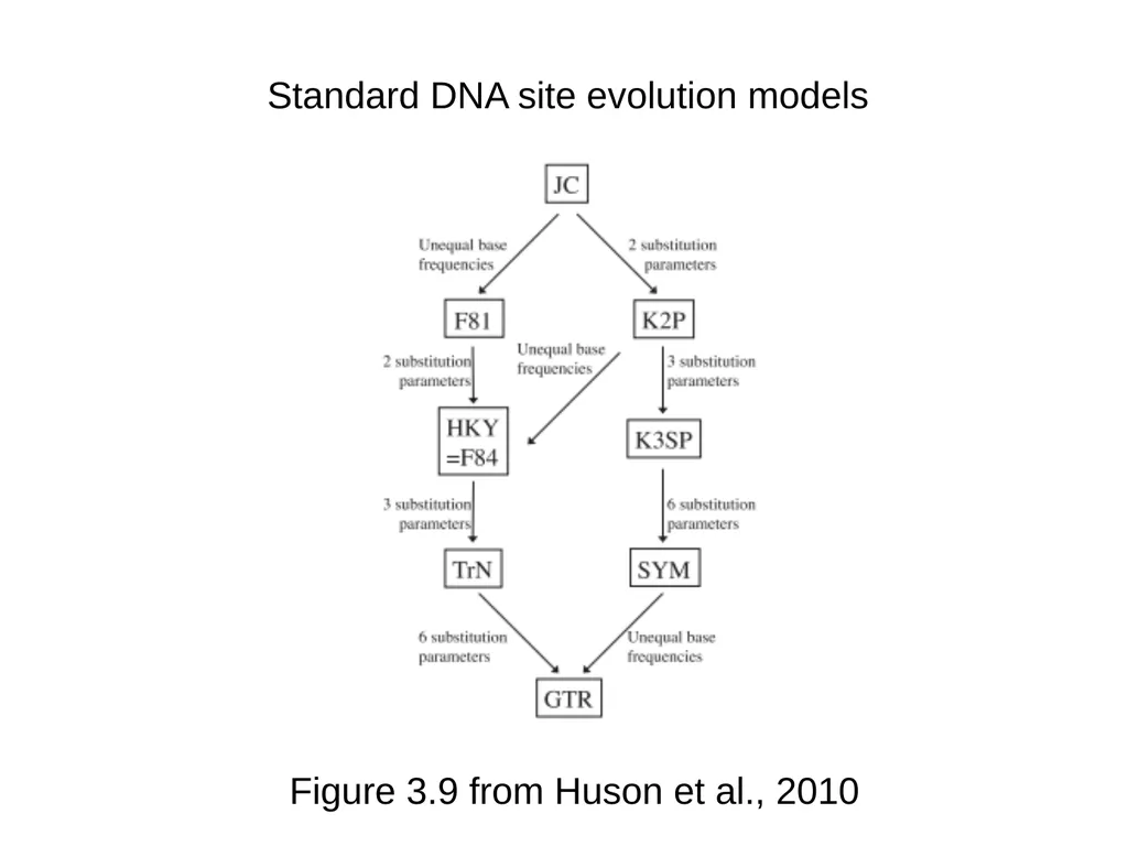
More complicated DNA sequence evolution models

See textbook Chapter 1, 8.1-8.2<br>
slide3. First… why unrooted trees? Remember that I said that most models of sequence evolution are time-reversible.
Hence the best we can do is to infer an unrooted tree.
Get used to drawing unrooted trees!
Get used to taking a rooted tree and drawing it without the root.
You can assume henceforth that I am always talking about unrooted trees – unless I say otherwise.
Also: in biology, most of the time, we expect binary rooted evolutionary trees (all internal nodes have two children), so the unrooted trees are also “binary” (all internal nodes have degree 3)<br>
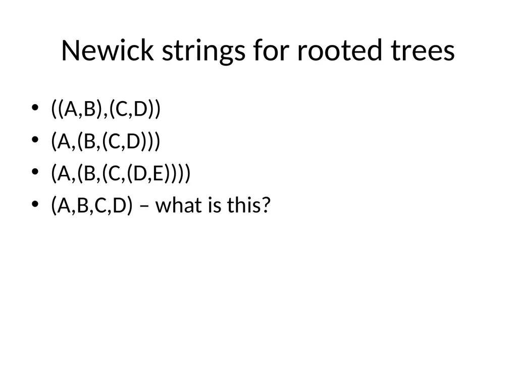
slide4. Newick strings for rooted trees ((A,B),(C,D))
(A,(B,(C,D)))
(A,(B,(C,(D,E))))
(A,B,C,D) – what is this?<br>
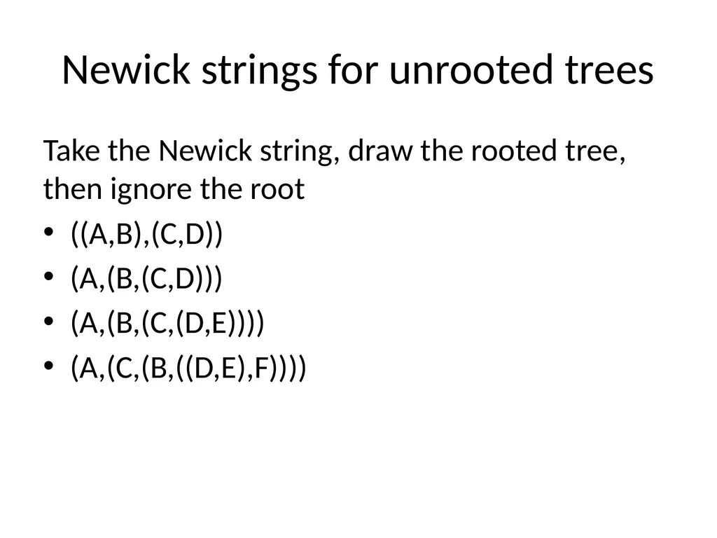
slide5. Newick strings for unrooted trees Take the Newick string, draw the rooted tree, then ignore the root
((A,B),(C,D))
(A,(B,(C,D)))
(A,(B,(C,(D,E))))
(A,(C,(B,((D,E),F))))<br>
slide6. Representations for unrooted quartet trees Instead of writing the Newick string, you can use something simpler:
AB|CD instead of ((A,B),(C,D))<br>
slide7. Class exercise Draw the rooted and unrooted trees given by Newick Strings
((A,B)(C,(D,E)))
(A,(B,(C,(E,D)))
(E,(D,((A,B),C)))<br>
slide8. Induced subtrees T is a tree with leaves labelled by set S
A is a subset of S
Question: What is T|A

Answer: Write T, erase every leaf not in A, and see what you get<br>
slide9. Q(T): the set of induced quartet trees Every unrooted tree T is uniquely defined by its set Q(T) of induced quartet trees
Typical task: given a Newick string, write down the unrooted tree, and then write down the set Q(T)<br>
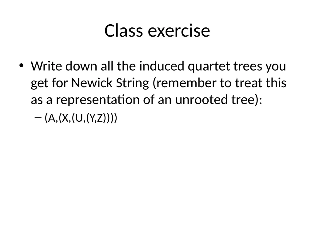
slide10. Class exercise Write down all the induced quartet trees you get for Newick String (remember to treat this as a representation of an unrooted tree):
(A,(X,(U,(Y,Z))))<br>
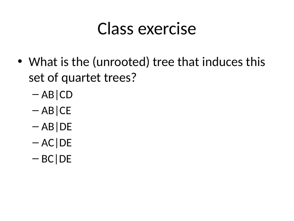
slide11. Class exercise What is the (unrooted) tree that induces this set of quartet trees?
AB|CD
AB|CE
AB|DE
AC|DE
BC|DE<br>
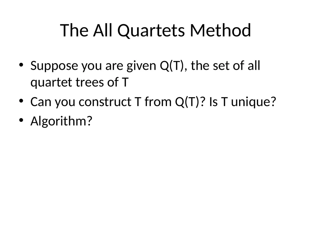
slide12. The All Quartets Method Suppose you are given Q(T), the set of all quartet trees of T
Can you construct T from Q(T)? Is T unique?
Algorithm?<br>
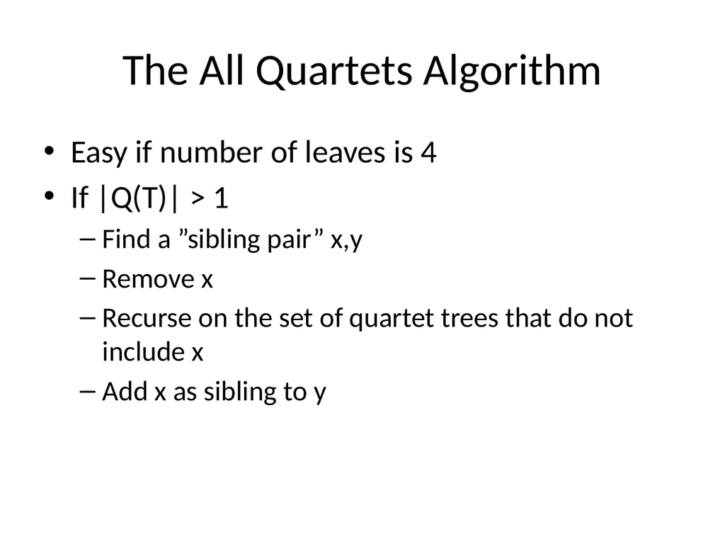
slide13. The All Quartets Algorithm Easy if number of leaves is 4
If |Q(T)| > 1
Find a ”sibling pair” x,y
Remove x
Recurse on the set of quartet trees that do not include x
Add x as sibling to y<br>
slide14. Warm-up to “Additive Distances” Suppose we now put non-negative branch lengths on the edges of the tree. We want to compute the matrix of leaf-to-leaf distances (computed by summing up branch lengths)
Do this calculation for a four-leaf binary tree you make up
Do it again, but make the internal branch length zero
Do this calculation for a four-leaf non-binary (star) tree<br>
slide15. Additive Matrices A square matrix D=[dij] is additive if and only if there is a tree T and edge-weighting w such that for all pairs i,j of leaves, dij is the path distance in T between i and j.

We note this by saying D corresponds to (T,w).<br>
slide16. Distances, metrics, additive matrices, dissimilarity matrices What is a distance (aka metric)?
symmetric, non-negative, zero on diagonal, and satisfies triangle inequality: see https://jeremykun.com/tag/triangle-inequality/
Is every additive matrix a distance?
What about Hamming distances?
What is a dissimilarity matrix? Satisfies nearly all the requirements for a distance, but not the triangle inequality. This is NEEDED in biological sequence analysis.<br>
slide17. Class exercise Write down the tree on four leaves {A,B,C,D}, given by the split AB|CD.

Set the internal edge length to 5, and all external edge lengths to 1.

What is the additive matrix for this tree?<br>
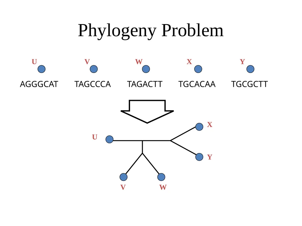
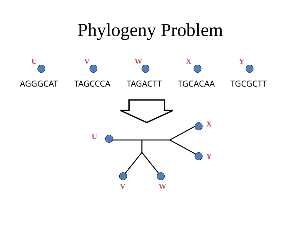
slide18. Phylogeny Problem TAGCCCA TAGACTT TGCACAA TGCGCTT AGGGCAT U V W X Y U V W X Y<br>
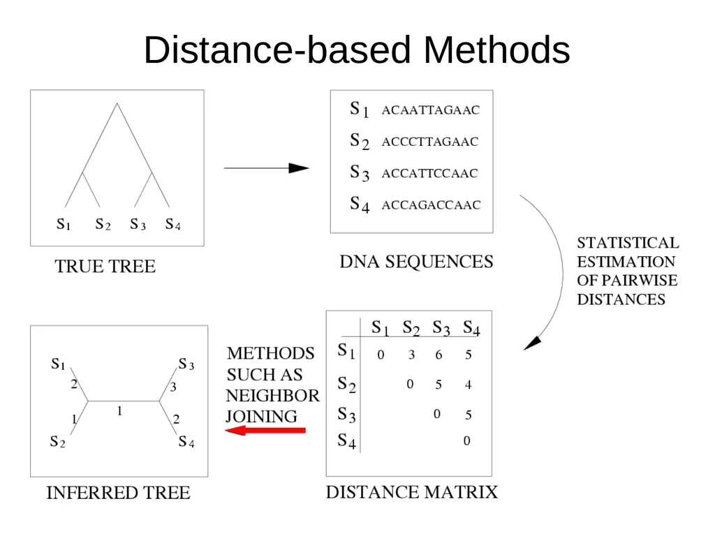
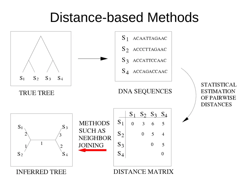
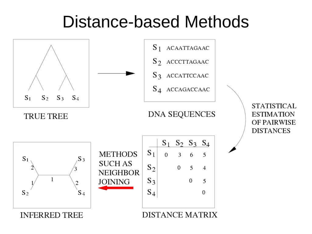
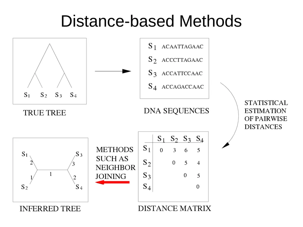
slide19. Distance-based Methods<br>
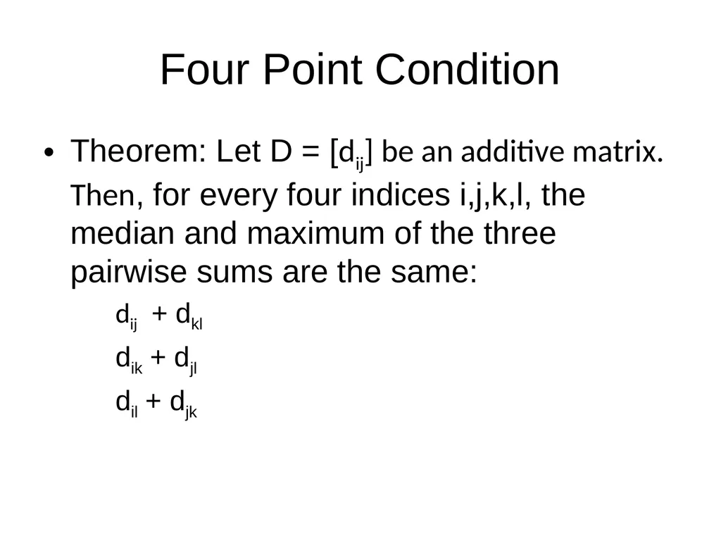
slide20. Four Point Condition Theorem: Let D = [dij] be an additive matrix. Then, for every four indices i,j,k,l, the median and maximum of the three pairwise sums are the same:
dij + dkl
dik + djl
dil + djk<br>
slide21. Proof of the Four Point Condition<br>
slide22. Using the Four Point Condition Given a 4x4 additive matrix D, can you find the tree T (and edge-weighting w) that corresponds to D?<br>
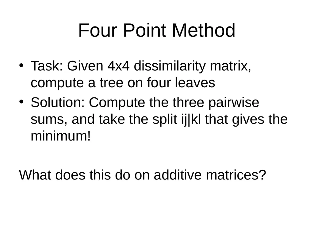
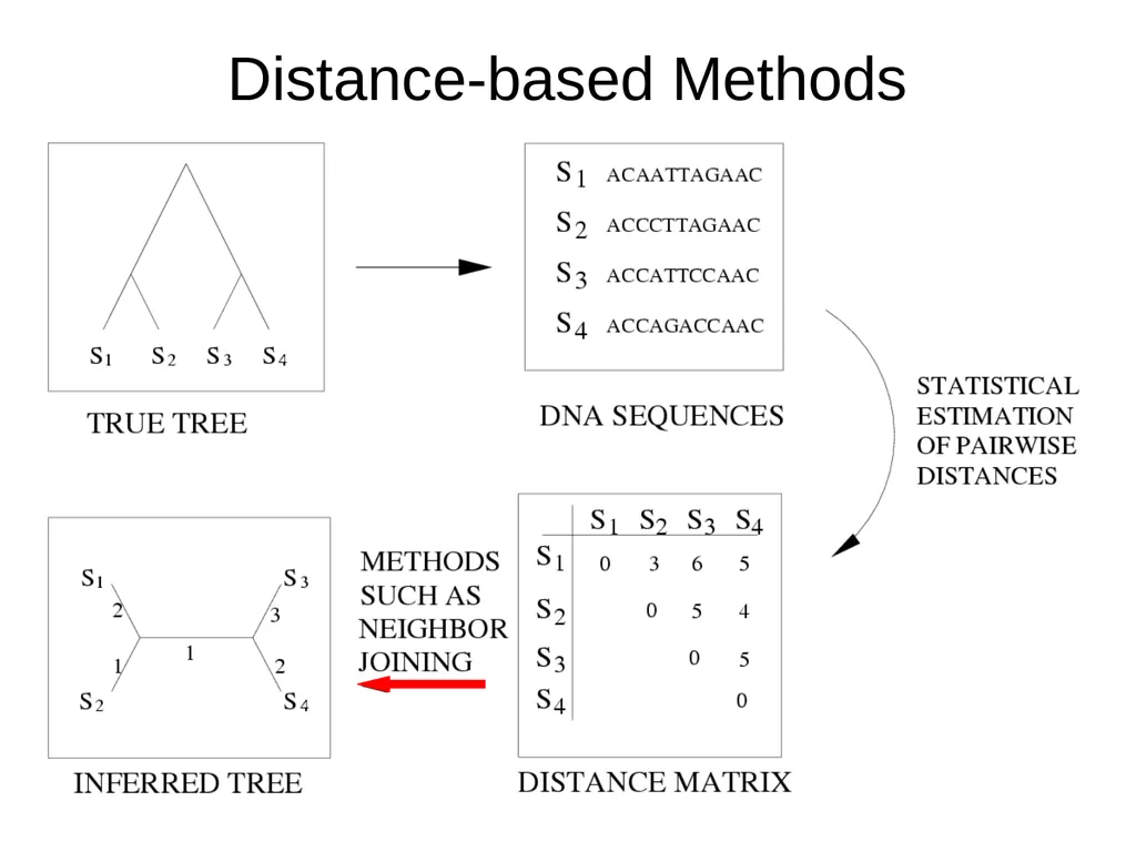
slide23. Four Point Method Task: Given 4x4 dissimilarity matrix, compute a tree on four leaves
Solution: Compute the three pairwise sums, and take the split ij|kl that gives the minimum!

What does this do on additive matrices?<br>
slide24. Using the Four Point Condition How would you construct a tree on a set of n>4 leaves, if you had an additive matrix?<br>
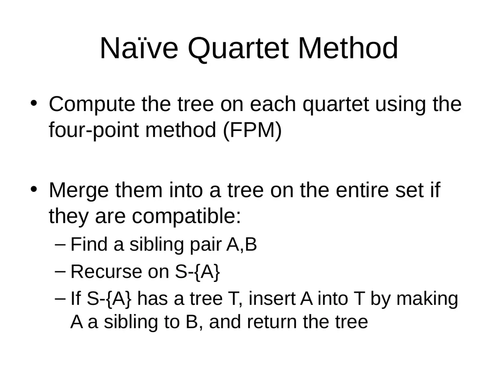
slide25. Naïve Quartet Method Compute the tree on each quartet using the four-point method (FPM)

Merge them into a tree on the entire set if they are compatible:
Find a sibling pair A,B
Recurse on S-{A}
If S-{A} has a tree T, insert A into T by making A a sibling to B, and return the tree<br>
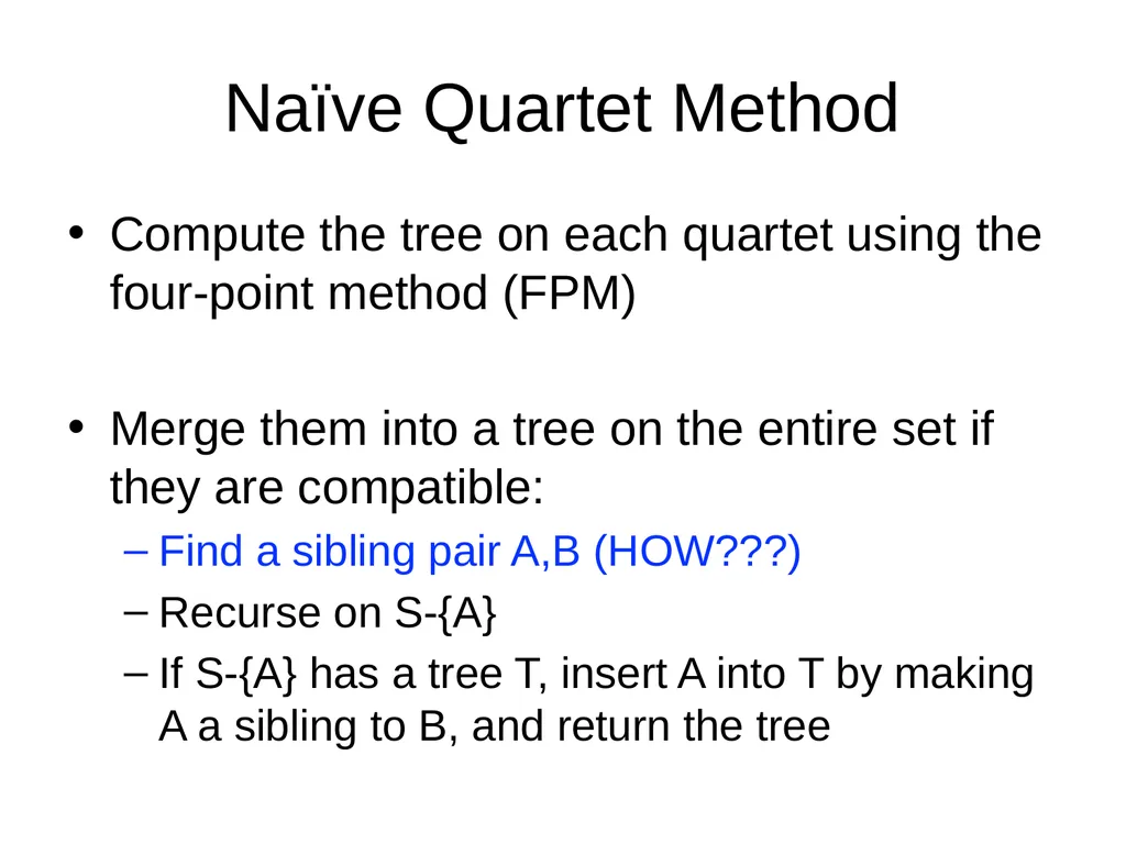
slide26. Naïve Quartet Method Compute the tree on each quartet using the four-point method (FPM)

Merge them into a tree on the entire set if they are compatible:
Find a sibling pair A,B (HOW???)
Recurse on S-{A}
If S-{A} has a tree T, insert A into T by making A a sibling to B, and return the tree<br>
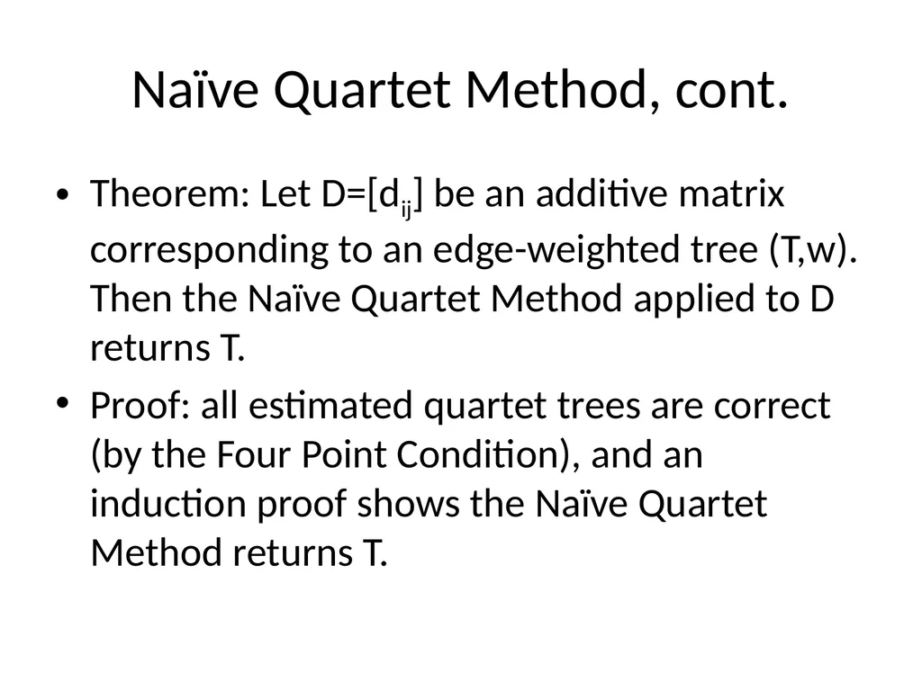
slide27. Naïve Quartet Method, cont. Theorem: Let D=[dij] be an additive matrix corresponding to an edge-weighted tree (T,w). Then the Naïve Quartet Method applied to D returns T.
Proof: all estimated quartet trees are correct (by the Four Point Condition), and an induction proof shows the Naïve Quartet Method returns T.<br>
slide28. Distance-based Methods<br>
slide29. Dissimilarity Matrices A square matrix that is symmetric and zero on the diagonal is called a dissimilarity matrix.
A dissimilarity matrix may not satisfy the triangle inequality.
In phylogenetics, the distance matrices we calculate are dissimilarity matrices.
Can we construct a tree from a dissimilarity matrix?<br>
slide30. Error tolerance for NQM Suppose every pairwise distance is estimated well enough (within f/2, for f the minimum length of any edge).
Then the Four Point Method returns the correct tree on every quartet.
And so all quartet trees are compatible, and NQM returns the true tree.<br>
slide31. Phylogeny estimation as a statistical inverse problem<br>
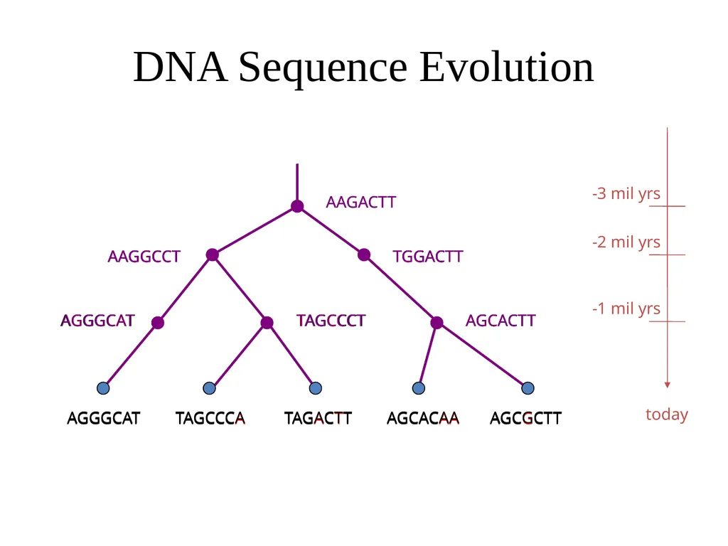
slide32. Estimation of evolutionary trees as a statistical inverse problem We can consider characters as properties that evolve down trees.
We observe the character states at the leaves, but the internal nodes of the tree also have states.
The challenge is to estimate the tree from the properties of the taxa at the leaves. This is enabled by characterizing the evolutionary process as accurately as we can.<br>
slide33. DNA Sequence Evolution<br>
slide34. Phylogeny Problem TAGCCCA TAGACTT TGCACAA TGCGCTT AGGGCAT U V W X Y U V W X Y<br>
slide35. Jukes-Cantor (1969) Model The model tree T is binary and has substitution probabilities p(e) on each edge e.
The state at the root is randomly drawn from {A,C,T,G} (nucleotides)
If a site (position) changes on an edge, it changes with equal probability to each of the remaining states.
The evolutionary process is Markovian.

More complex models (such as the General Time Reversible model, or the General Markov model) are also considered, often with little change to the theory.<br>
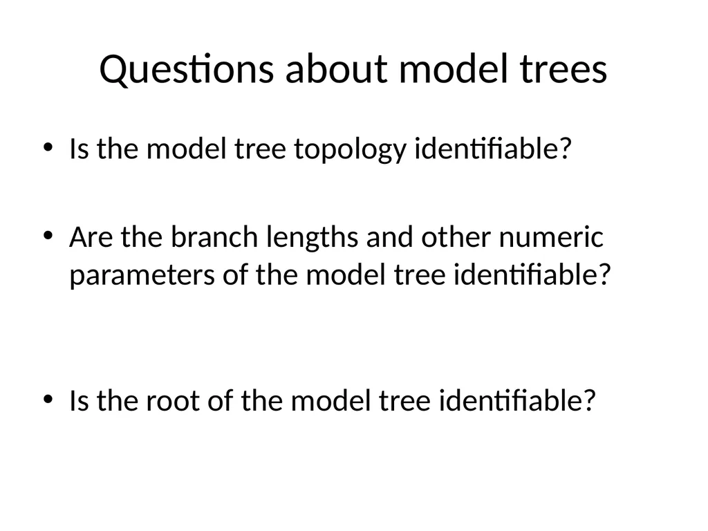
slide36. Questions about model trees Is the model tree topology identifiable? – yes

Are the branch lengths and other numeric parameters of the model tree identifiable? – yes

Is the root of the model tree identifiable? – no<br>
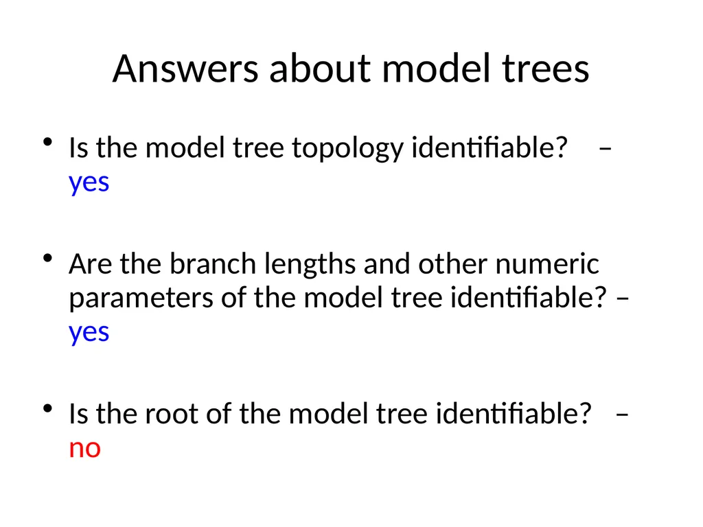
slide37. Answers about model trees Is the model tree topology identifiable? – yes

Are the branch lengths and other numeric parameters of the model tree identifiable? – yes

Is the root of the model tree identifiable? – no<br>
slide38. Distance-based Methods<br>
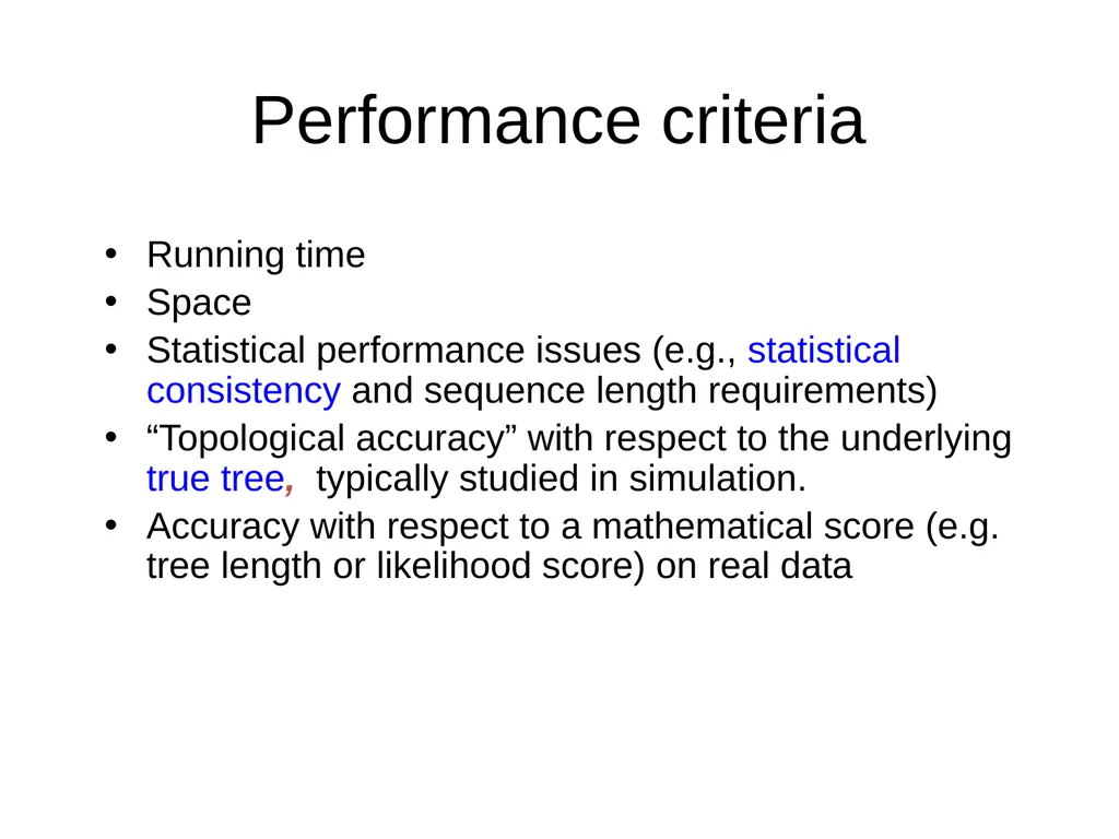
slide39. Performance criteria Running time
Space
Statistical performance issues (e.g., statistical consistency and sequence length requirements)
“Topological accuracy” with respect to the underlying true tree, typically studied in simulation.
Accuracy with respect to a mathematical score (e.g. tree length or likelihood score) on real data<br>
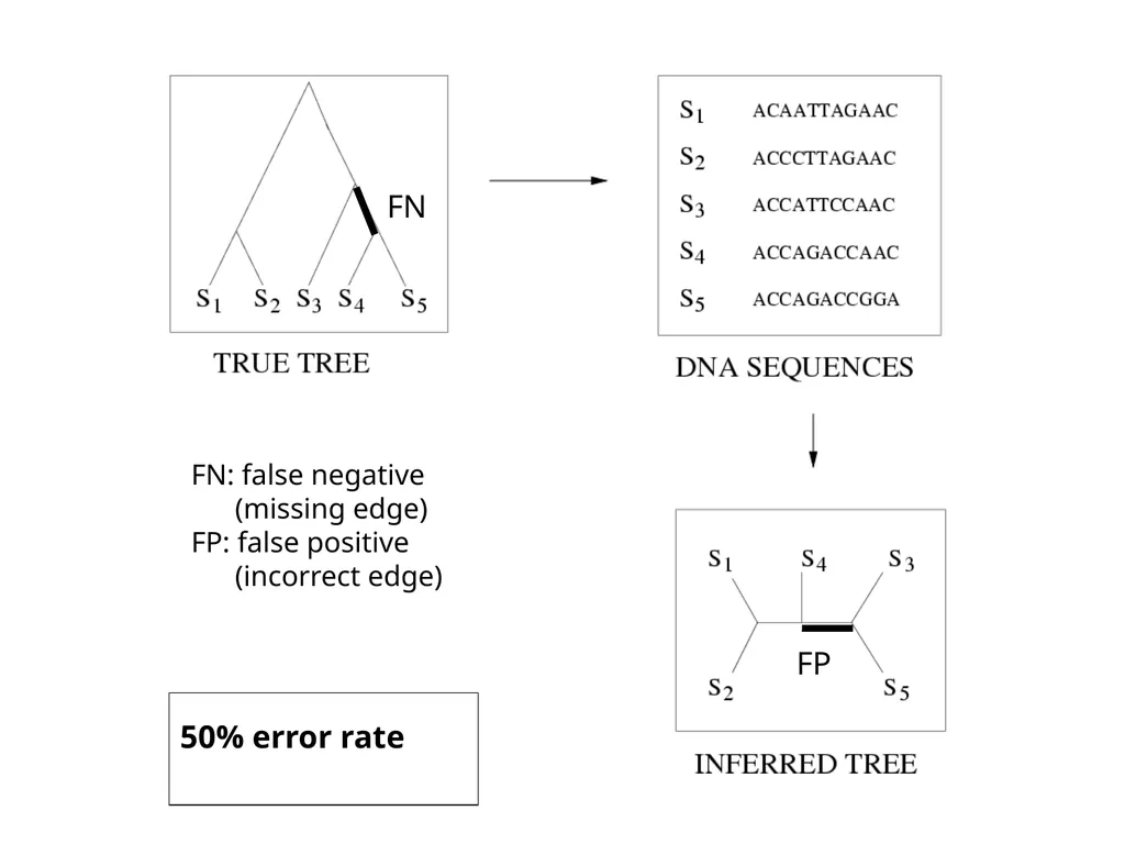
slide40. FN: false negative
(missing edge)
FP: false positive
(incorrect edge) FN FP 50% error rate<br>
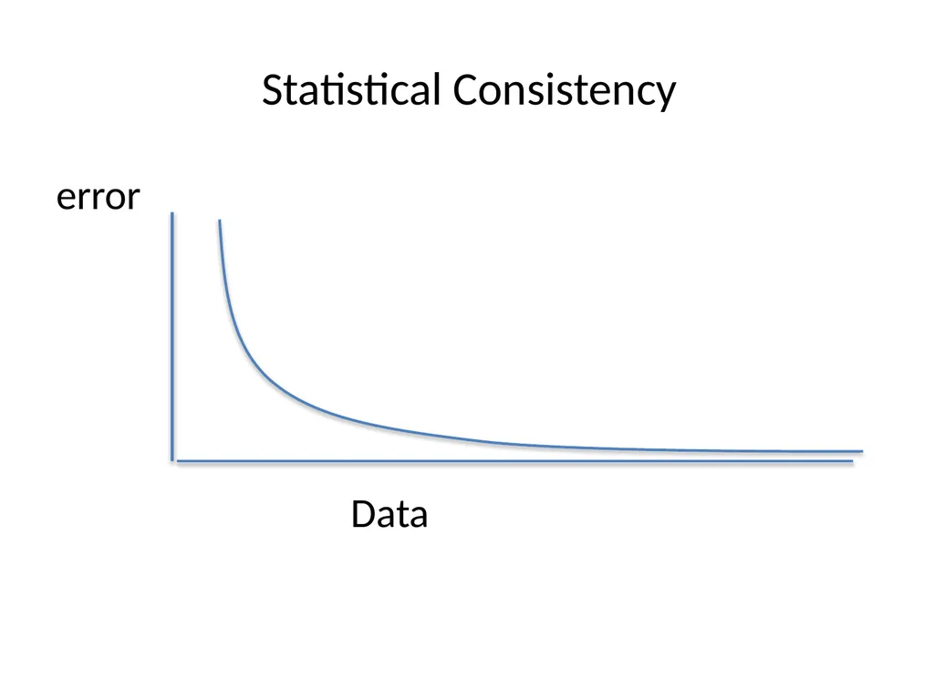
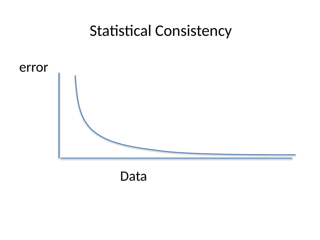
slide41. Statistical Consistency error Data<br>
slide42. Statistical models Simple example: coin tosses.
Suppose your coin has probability p of turning up heads, and you want to estimate p. How do you do this?<br>
slide43. Estimating p Toss coin repeatedly
Let your estimate q be the fraction of the time you get a head

Obvious observation: q will approach p as the number of coin tosses increases
This algorithm is a statistically consistent estimator of p. That is, your error |q-p| goes to 0 (with high probability) as the number of coin tosses increases.<br>
slide44. Another estimation problem Suppose your coin is biased either towards heads or tails (so that p is not 1/2).
How do you determine which type of coin you have?

Same algorithm, but say “heads” if q>1/2, and “tails” if q<1/2. For large enough number of coin tosses, your answer will be correct with high probability.<br>
slide45. Phylogeny Estimation Simplest type of data: presence/absence of a property (e.g., has wings, has hair, has a particular amino acid)
Treat this as binary character evolution, with 0 representing absence and 1 representing presence.
How do we model the evolution of these binary characters?<br>
slide46. Jukes-Cantor (1969) Model The model tree T is binary and has substitution probabilities p(e) on each edge e.
The state at the root is randomly drawn from {A,C,T,G} (nucleotides)
If a site (position) changes on an edge, it changes with equal probability to each of the remaining states.
The evolutionary process is Markovian.

More complex models (such as the General Time Reversible model, or the General Markov model) are also considered, often with little change to the theory.<br>
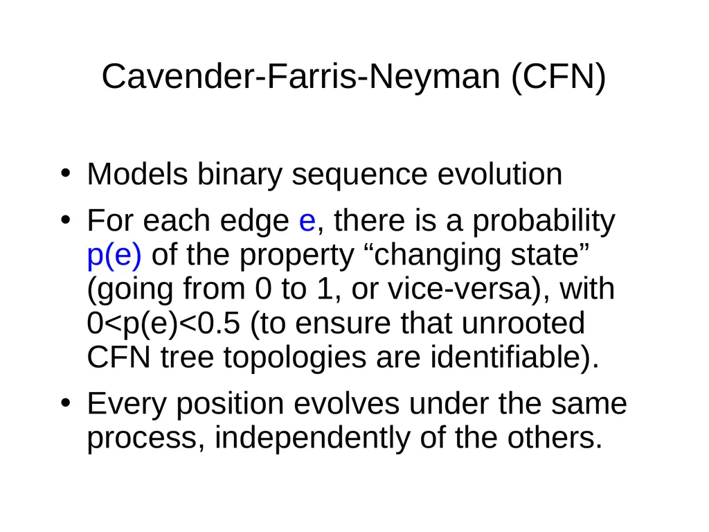
slide47. Cavender-Farris-Neyman (CFN) Models binary sequence evolution
For each edge e, there is a probability p(e) of the property “changing state” (going from 0 to 1, or vice-versa), with 0<p(e)<0.5 (to ensure that unrooted CFN tree topologies are identifiable).
Every position evolves under the same process, independently of the others.<br>
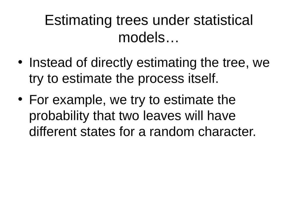
slide48. Estimating trees under statistical models… Instead of directly estimating the tree, we try to estimate the process itself.
For example, we try to estimate the probability that two leaves will have different states for a random character.<br>
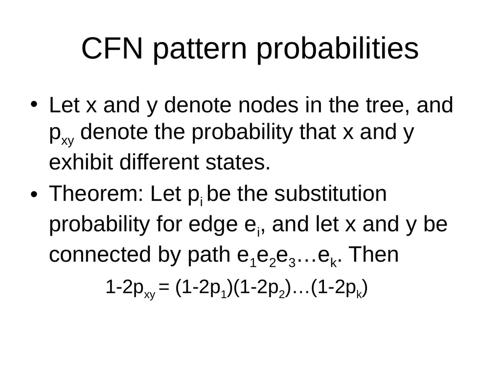
slide49. CFN pattern probabilities Let x and y denote nodes in the tree, and pxy denote the probability that x and y exhibit different states.
Theorem: Let pi be the substitution probability for edge ei, and let x and y be connected by path e1e2e3…ek. Then
1-2pxy = (1-2p1)(1-2p2)…(1-2pk)<br>
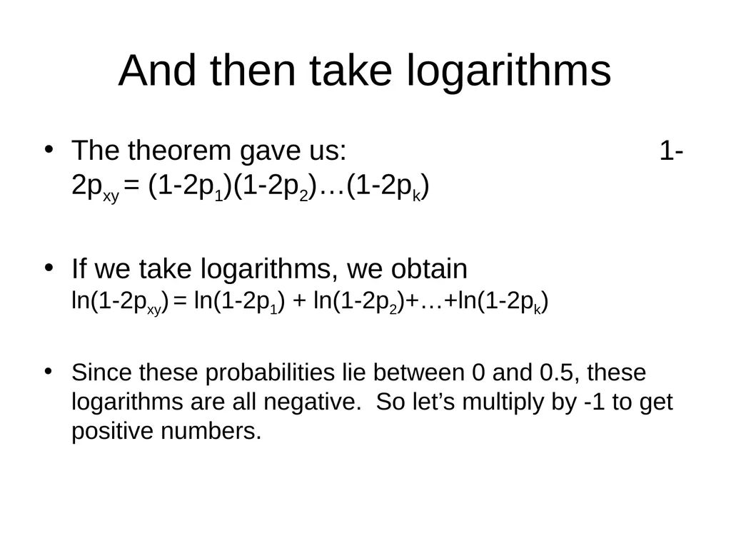
slide50. And then take logarithms The theorem gave us: 1-2pxy = (1-2p1)(1-2p2)…(1-2pk)

If we take logarithms, we obtain ln(1-2pxy) = ln(1-2p1) + ln(1-2p2)+…+ln(1-2pk)

Since these probabilities lie between 0 and 0.5, these logarithms are all negative. So let’s multiply by -1 to get positive numbers.<br>
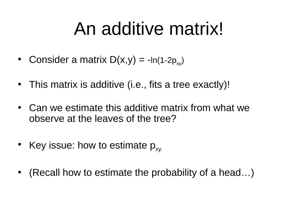
slide51. An additive matrix! Consider a matrix D(x,y) = -ln(1-2pxy)

This matrix is additive (i.e., fits a tree exactly)!

Can we estimate this additive matrix from what we observe at the leaves of the tree?

Key issue: how to estimate pxy.

(Recall how to estimate the probability of a head…)<br>
slide52. Distance-based Methods<br>
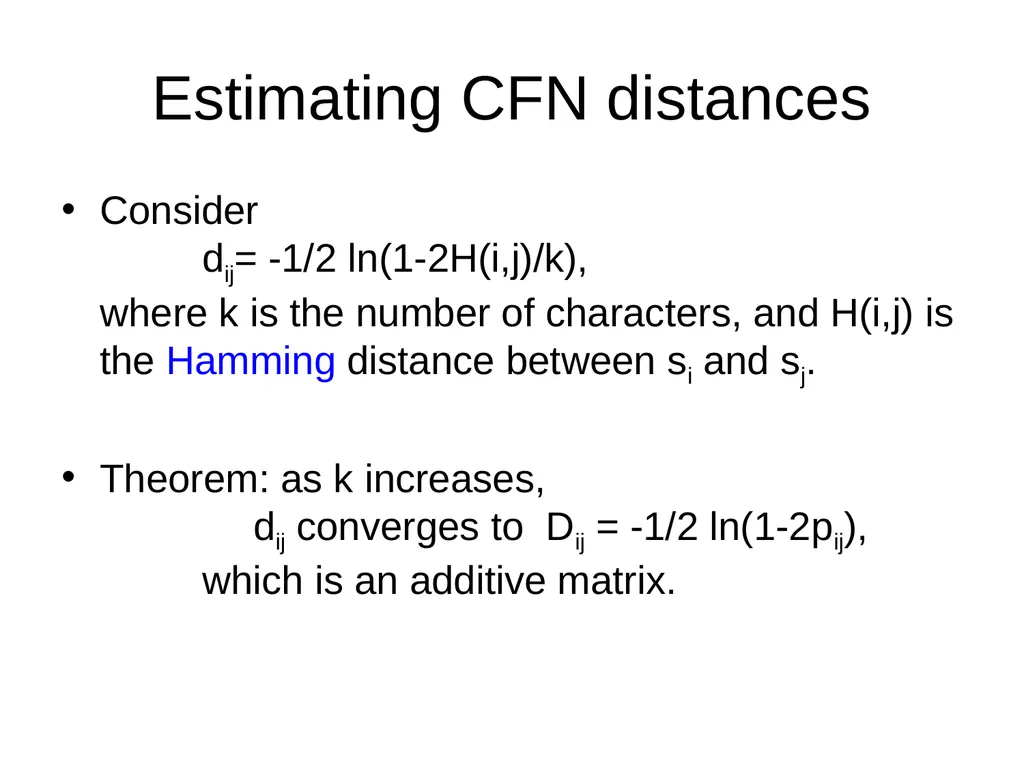
slide53. Estimating CFN distances Consider dij= -1/2 ln(1-2H(i,j)/k), where k is the number of characters, and H(i,j) is the Hamming distance between si and sj.

Theorem: as k increases, dij converges to Dij = -1/2 ln(1-2pij), which is an additive matrix.<br>
slide54. Four Point Method (FPM) Task: Given 4x4 dissimilarity matrix, compute a tree on four leaves
Solution: Compute the three pairwise sums, and take the split ij|kl that gives the minimum!
When is this guaranteed accurate?<br>
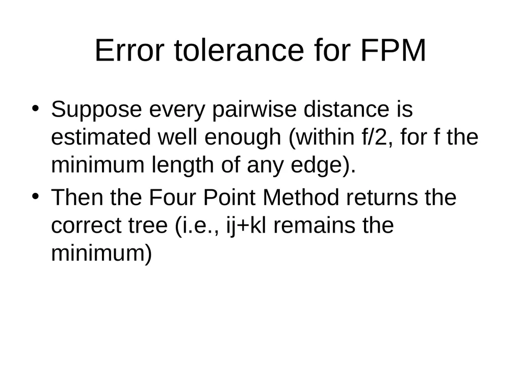
slide55. Error tolerance for FPM Suppose every pairwise distance is estimated well enough (within f/2, for f the minimum length of any edge).
Then the Four Point Method returns the correct tree (i.e., ij+kl remains the minimum)<br>
slide56. Naïve Quartet Method (NQM) Compute the tree on each quartet using the four-point method
Merge them into a tree on the entire set if they are compatible:
Find a sibling pair A,B
Recurse on S-{A}
If S-{A} has a tree T, insert A into T by making A a sibling to B, and return the tree<br>
slide57. Error tolerance for NQM Suppose every pairwise distance is estimated well enough (within f/2, for f the minimum length of any edge).
Then the Four Point Method returns the correct tree on every quartet.
And so all quartet trees are compatible, and NQM returns the true tree.<br>
slide58. In other words: The NQM method is statistically consistent methods for estimating CFN trees!
Plus it is polynomial time!<br>
slide59. Statistical Consistency error Data<br>
slide60. What about DNA sequence evolution? The proof of statistical consistency for the NQM under the CFN model only really depended on the guarantee that CFN estimated distances converge, as the sequence length increase, to an additive matrix.
What about DNA sequence evolution models?<br>
slide61. Jukes-Cantor (1969) Model The model tree T is binary and has substitution probabilities p(e) on each edge e.
The state at the root is randomly drawn from {A,C,T,G} (nucleotides)
If a site (position) changes on an edge, it changes with equal probability to each of the remaining states.
The evolutionary process is Markovian.

More complex models (such as the General Time Reversible model, or the General Markov model) are also considered, often with little change to the theory.<br>
slide62. Distance-based Methods<br>
slide63. Jukes-Cantor Tree Estimation Step 1: Compute Hamming distances
Step 2: Correct the Hamming distances, using the JC distance calculation
Step 3: Use NQM to construct the tree<br>
slide64. In other words: Theorem: The NQM method is statistically consistent methods for estimating JC trees, and uses polynomial time! 
Notes:
This is true for other models – all you need is a statistically consistent technique to estimate an additive matrix that corresponds to an edge-weighting of the model tree.
This is also true for other distance-based methods (e.g., neighbor joining).<br>
slide65. Standard DNA site evolution models Figure 3.9 from Huson et al., 2010<br>