
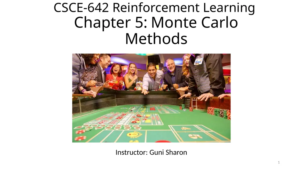
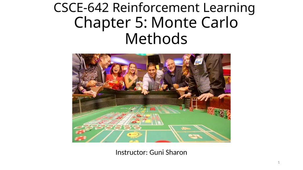
CSCE-642 Reinforcement Learning Chapter 5: Monte
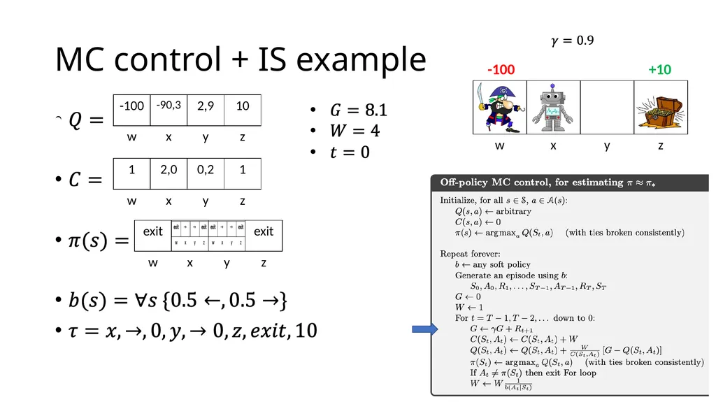
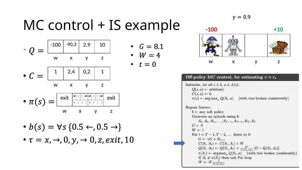
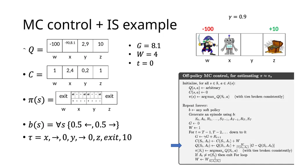
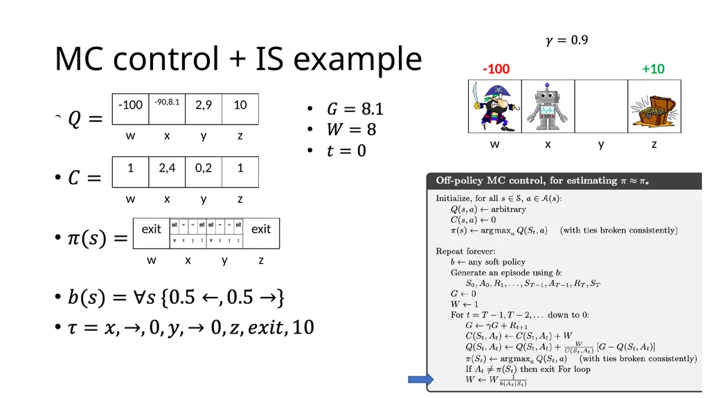
Description: CSCE-642 Reinforcement Learning Chapter 5: Monte Carlo Methods Instructor: Guni Sharon 1 CSCE-689, Reinforcement Learning Stateless decision process Markov decision process Solving MDPs (offline) Dynamic programming Monte-Carlo Temporal
Related Topics
Download Presentation
"CSCE-642 Reinforcement Learning Chapter 5: Monte" is the property of its rightful owner. Permission is granted to download and print the materials on this website for personal, non-commercial use only, and to display it on your personal computer provided you do not modify the materials and that you retain all copyright notices contained in the materials. By downloading content from our website, you accept the terms of this agreement.
Presentation Transcript
slide1. CSCE-642 Reinforcement Learning
Chapter 5: Monte Carlo Methods Instructor: Guni Sharon 1<br>
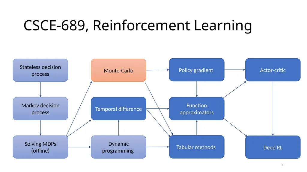
slide2. CSCE-689, Reinforcement Learning Stateless decision process Markov decision process Solving MDPs (offline) Dynamic programming Monte-Carlo Temporal difference Tabular methods Function approximators Policy gradient Deep RL Actor-critic 2<br>
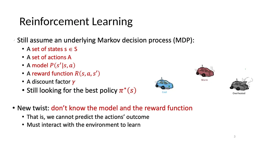
slide3. Reinforcement Learning 3<br>
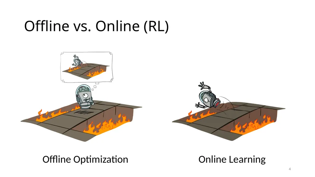
slide4. Offline vs. Online (RL) Offline Optimization Online Learning 4<br>
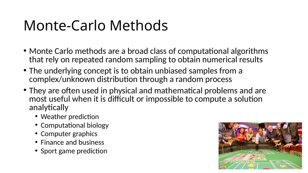
slide5. Monte-Carlo Methods Monte Carlo methods are a broad class of computational algorithms that rely on repeated random sampling to obtain numerical results
The underlying concept is to obtain unbiased samples from a complex/unknown distribution through a random process
They are often used in physical and mathematical problems and are most useful when it is difficult or impossible to compute a solution analytically
Weather prediction
Computational biology
Computer graphics
Finance and business
Sport game prediction 5<br>
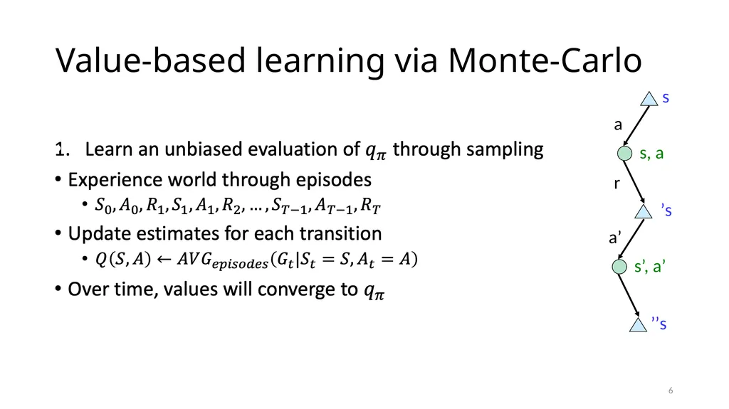
slide6. Value-based learning via Monte-Carlo r 6<br>
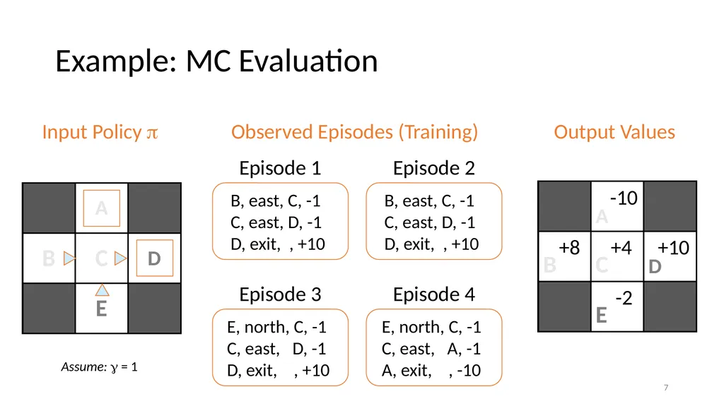
slide7. Example: MC Evaluation Input Policy Assume: = 1 Observed Episodes (Training) Output Values B, east, C, -1
C, east, D, -1
D, exit, , +10 B, east, C, -1
C, east, D, -1
D, exit, , +10 E, north, C, -1
C, east, A, -1
A, exit, , -10 Episode 1 Episode 2 Episode 3 Episode 4 E, north, C, -1
C, east, D, -1
D, exit, , +10 +8 +4 +10 -10 -2 7<br>
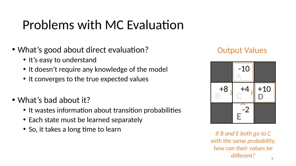
slide8. Problems with MC Evaluation What’s good about direct evaluation?
It’s easy to understand
It doesn’t require any knowledge of the model
It converges to the true expected values
What’s bad about it?
It wastes information about transition probabilities
Each state must be learned separately
So, it takes a long time to learn Output Values +8 +4 +10 -10 -2 If B and E both go to C with the same probability, how can their values be different? 8<br>
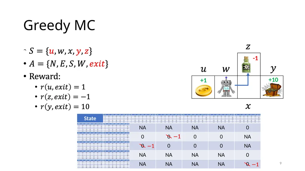
slide9. Greedy MC +10 -1 +1 9<br>
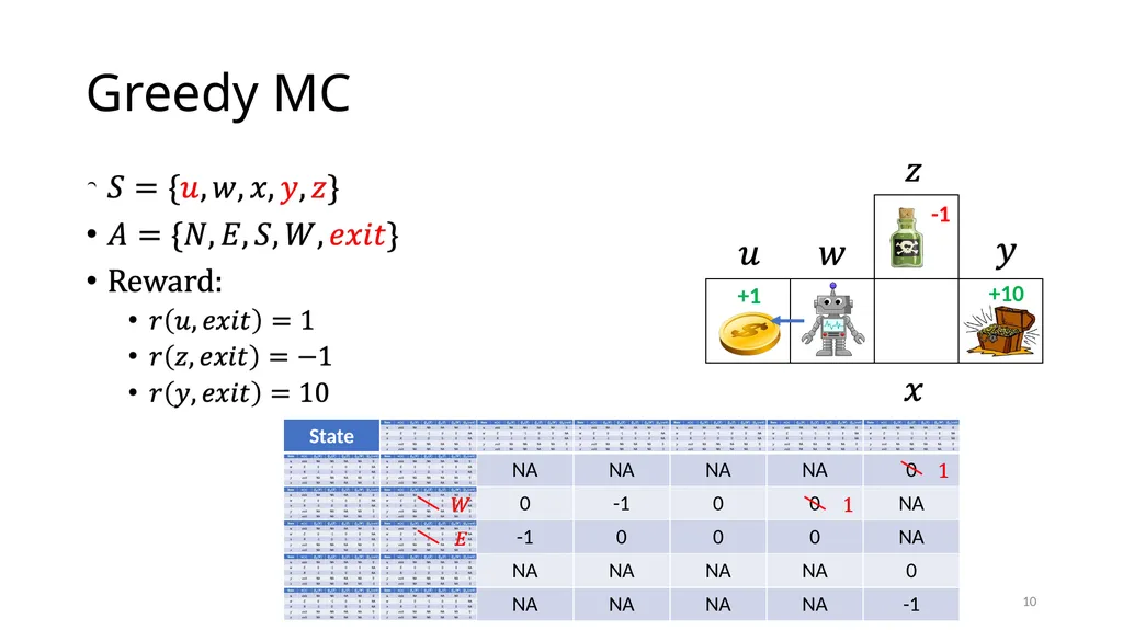
slide10. Greedy MC +10 -1 +1 10<br>
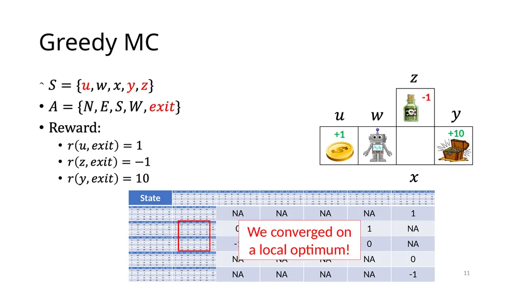
slide11. Greedy MC +10 -1 +1 We converged on a local optimum! 11<br>
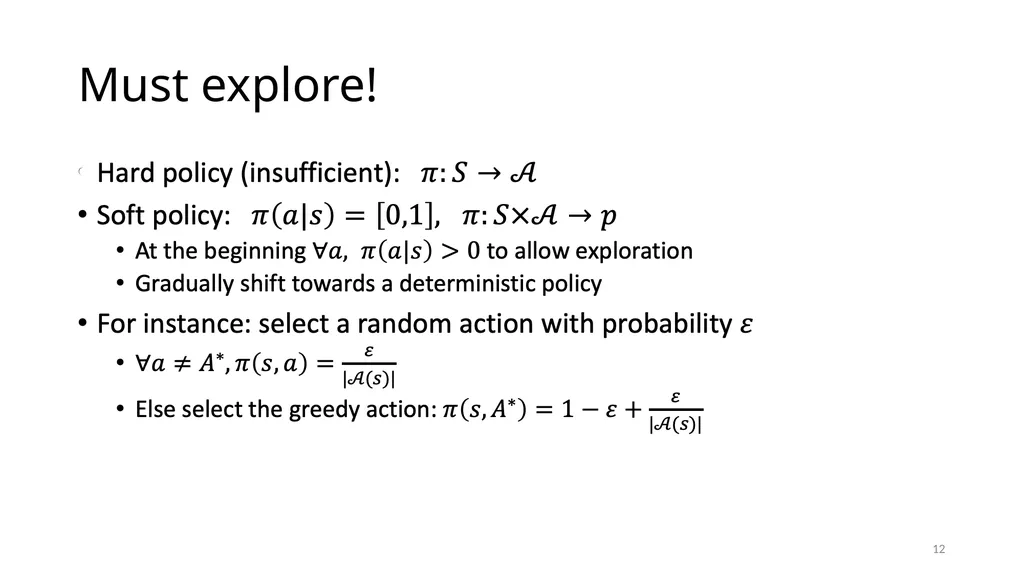
slide12. Must explore! 12<br>
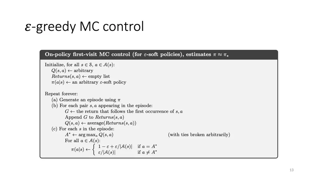
slide13. 13<br>
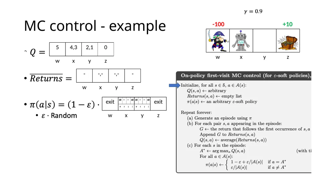
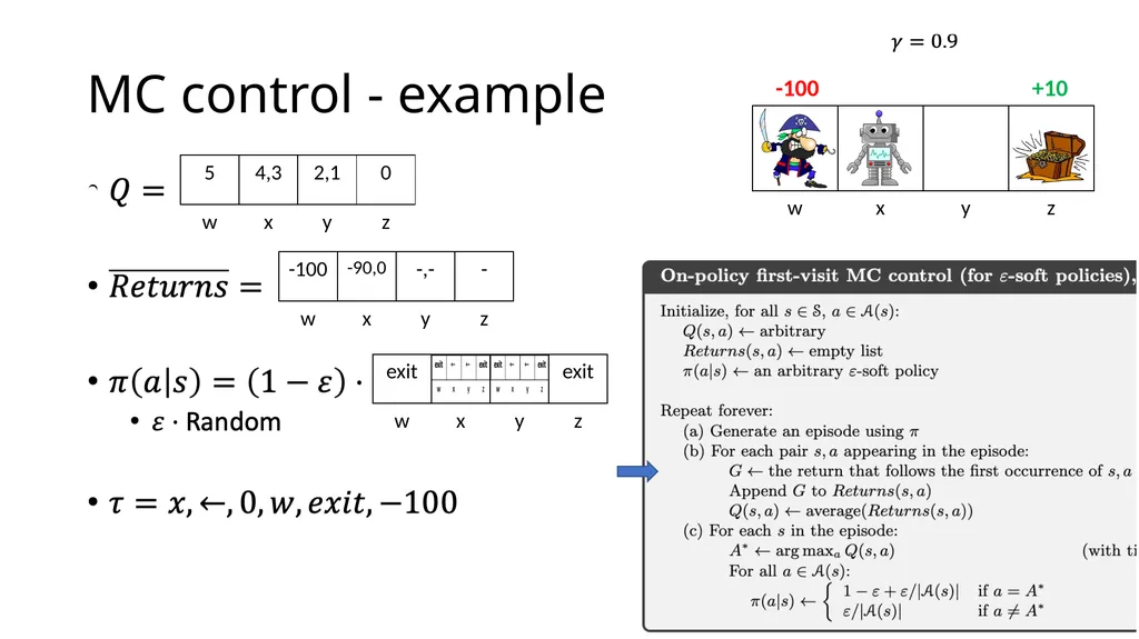
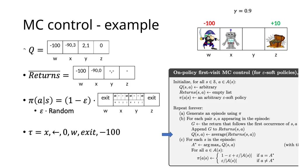
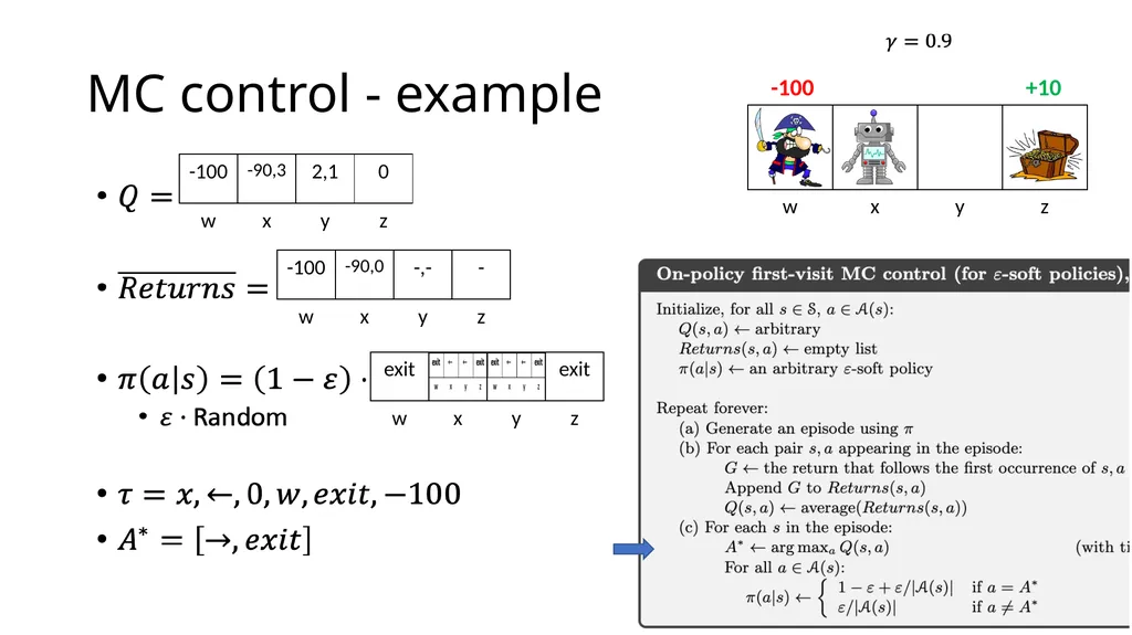
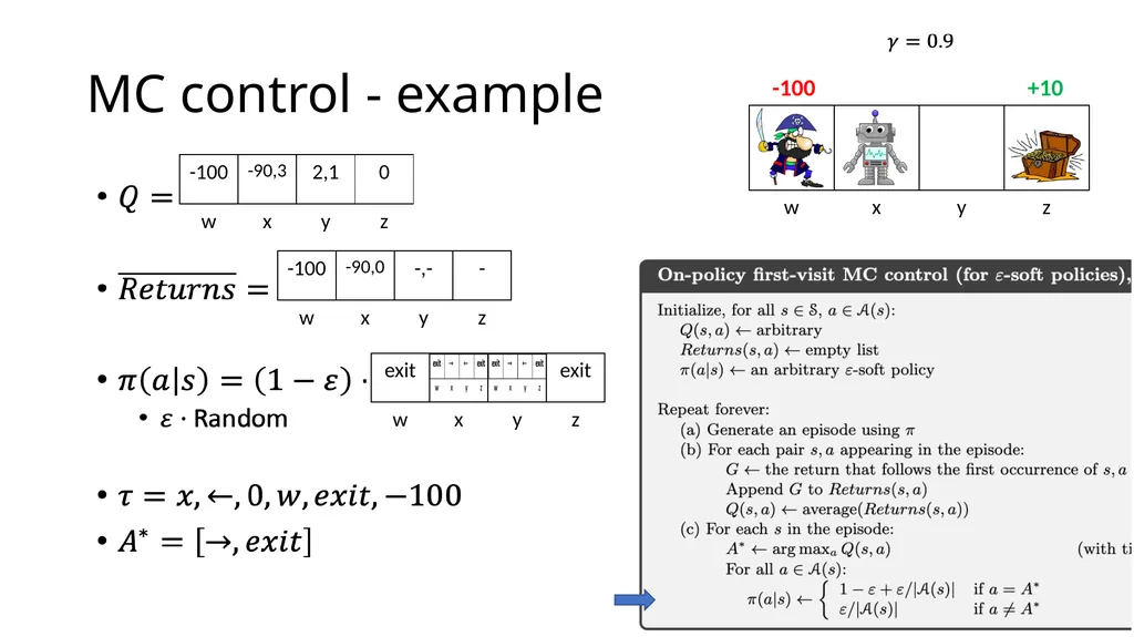
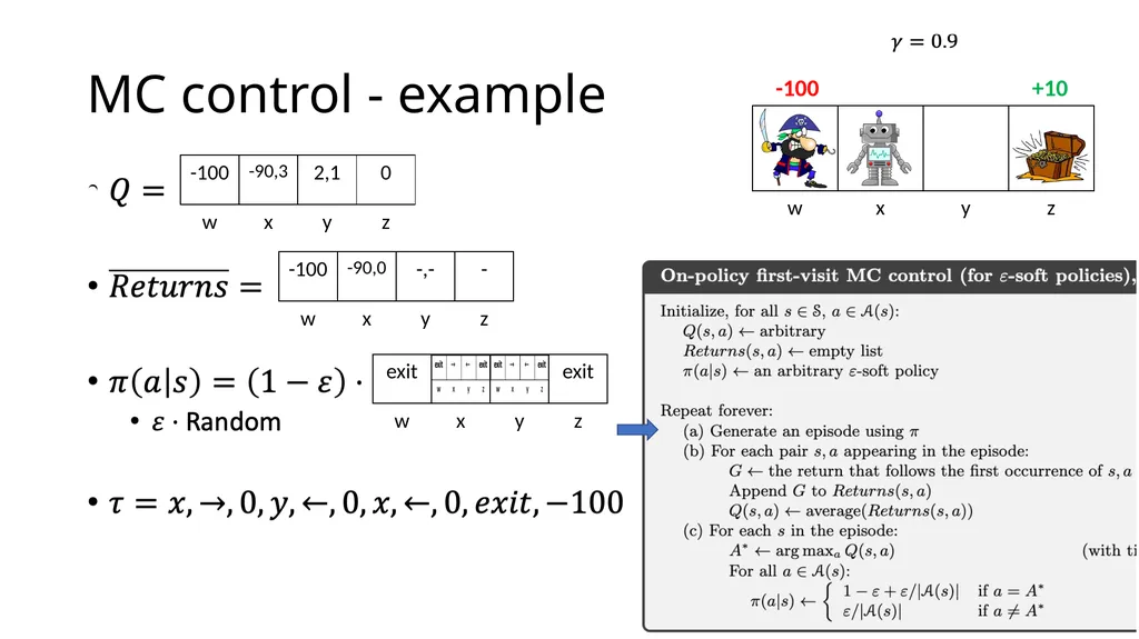
slide14. MC control - example +10 -100 14<br>
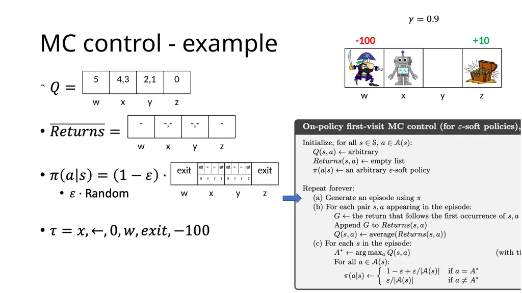
slide15. MC control - example +10 -100 15<br>
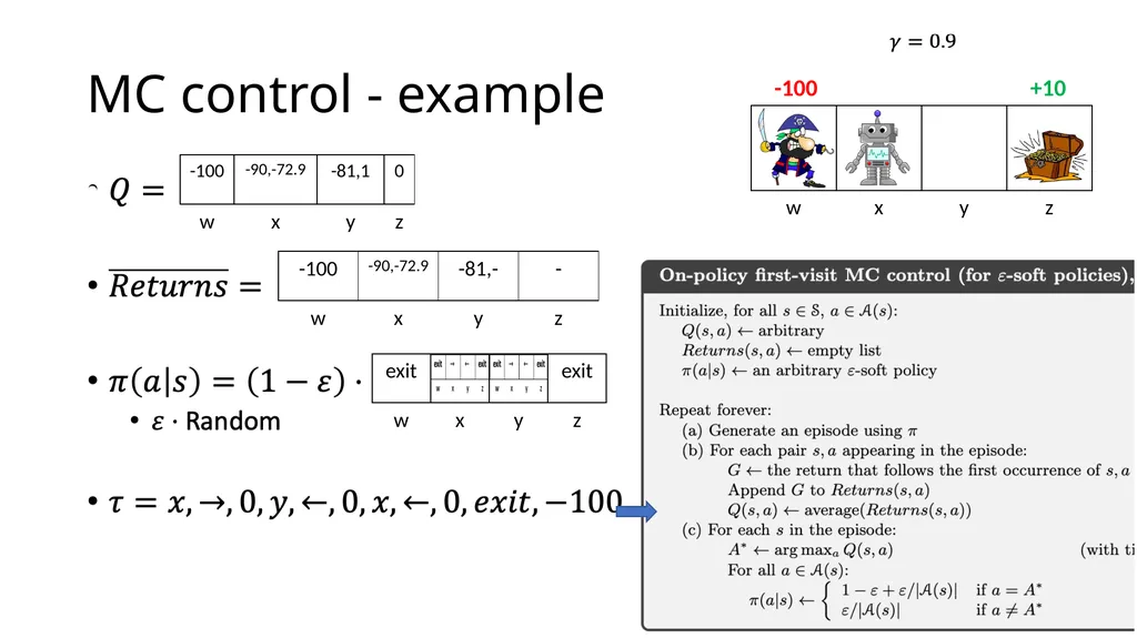
slide16. MC control - example +10 -100 16<br>
slide17. MC control - example +10 -100 17<br>
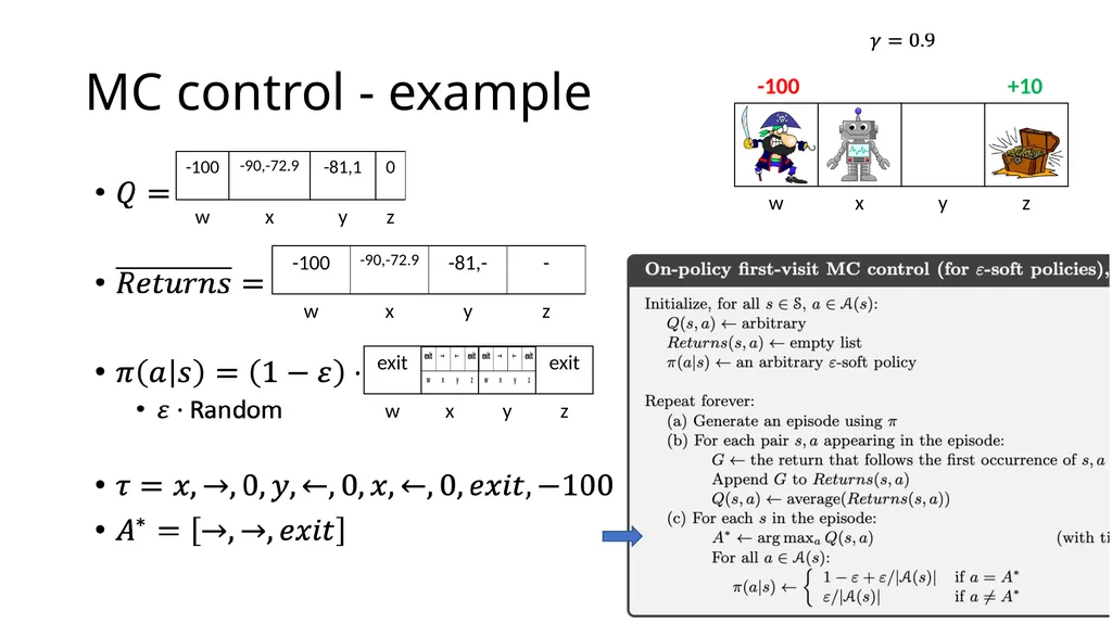
slide18. MC control - example +10 -100 18<br>
slide19. MC control - example +10 -100 19<br>
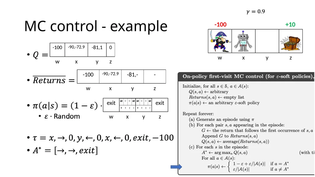
slide20. MC control - example +10 -100 20<br>
slide21. MC control - example +10 -100 21<br>
slide22. MC control - example +10 -100 22<br>
slide23. MC control - example +10 -100 23<br>
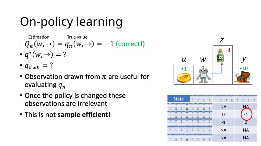
slide24. On-policy learning +10 -1 +1 24 Estimation True value<br>
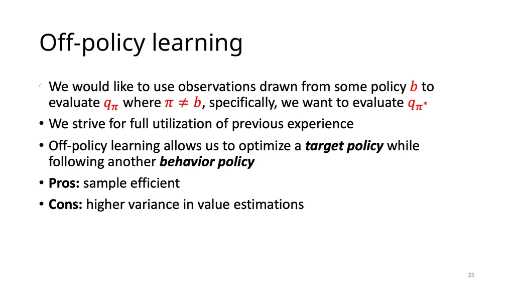
slide25. Off-policy learning 25<br>
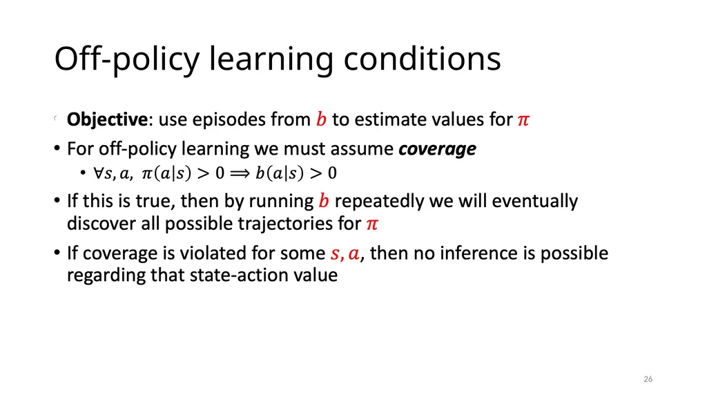
slide26. Off-policy learning conditions 26<br>
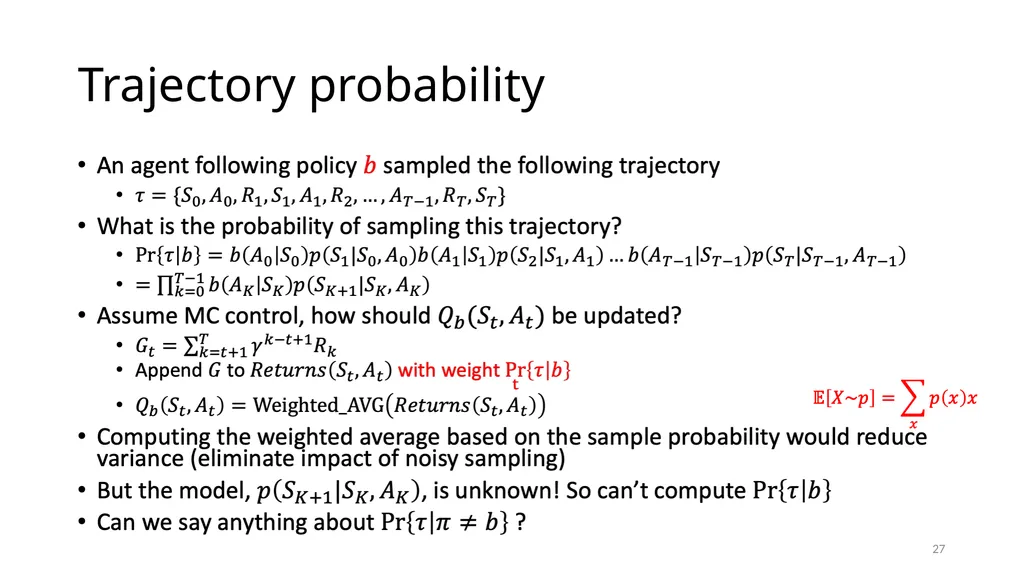
slide27. Trajectory probability 27<br>
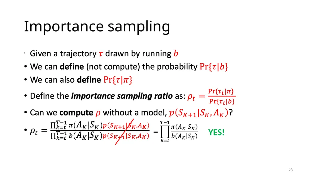
slide28. Importance sampling YES! 28<br>
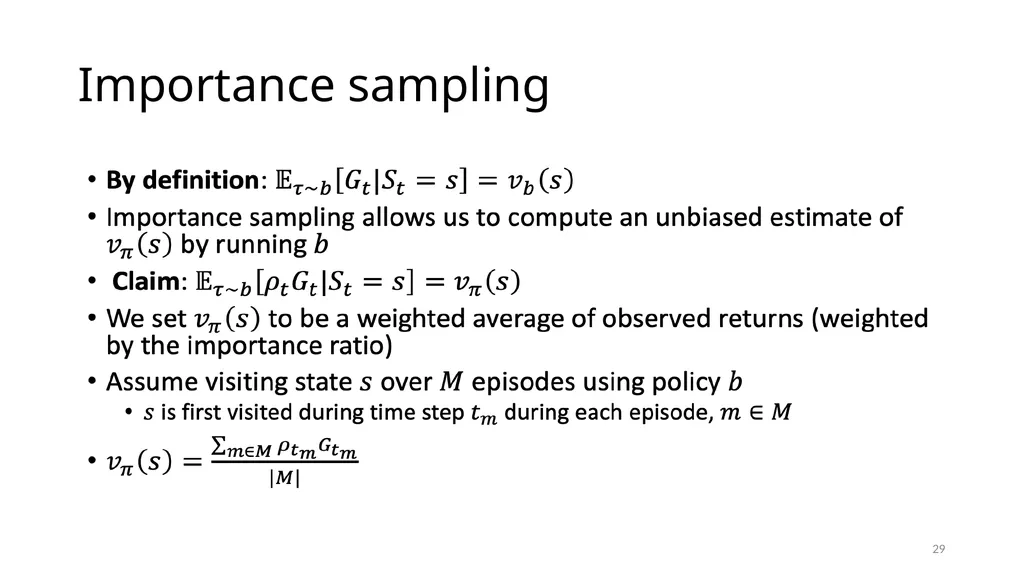
slide29. Importance sampling 29<br>
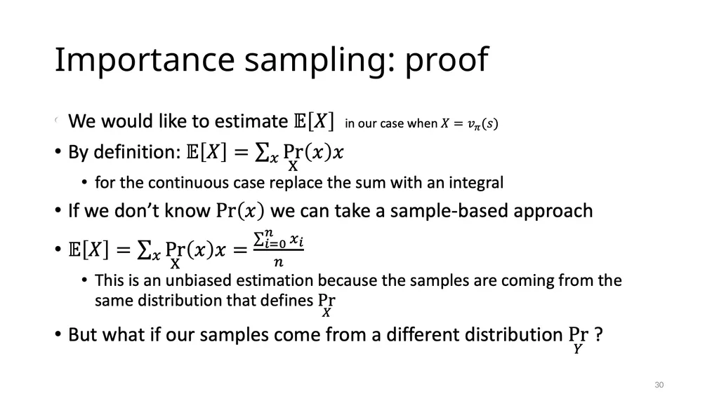
slide30. Importance sampling: proof 30<br>
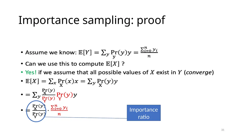
slide31. Importance sampling: proof 31 Importance ratio<br>
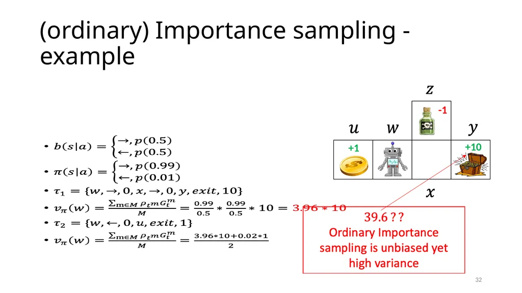
slide32. (ordinary) Importance sampling - example +10 -1 +1 32<br>
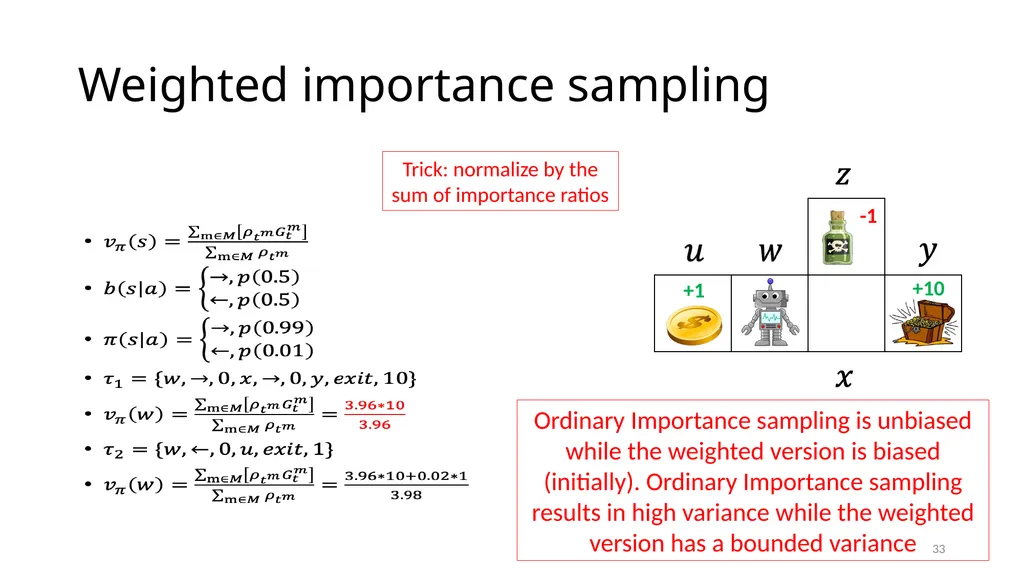
slide33. Weighted importance sampling +10 -1 +1 Ordinary Importance sampling is unbiased while the weighted version is biased (initially). Ordinary Importance sampling results in high variance while the weighted version has a bounded variance Trick: normalize by the sum of importance ratios 33<br>
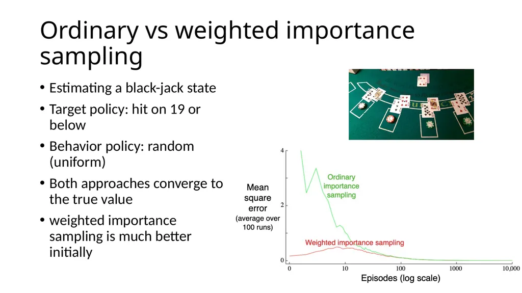
slide34. Ordinary vs weighted importance sampling Estimating a black-jack state
Target policy: hit on 19 or below
Behavior policy: random (uniform)
Both approaches converge to the true value
weighted importance sampling is much better initially 34<br>
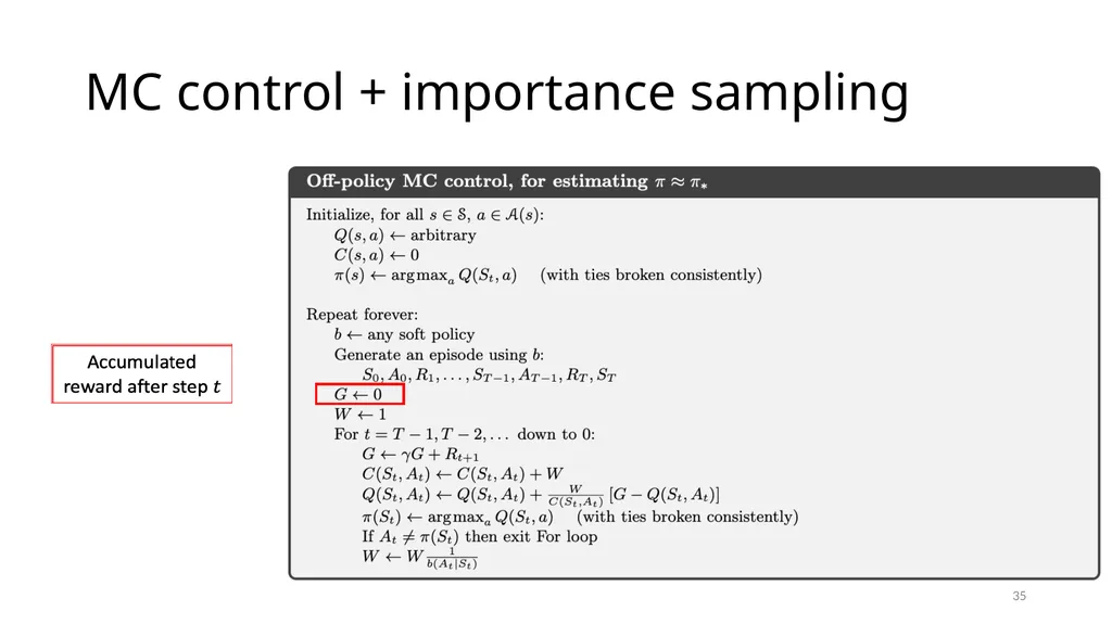
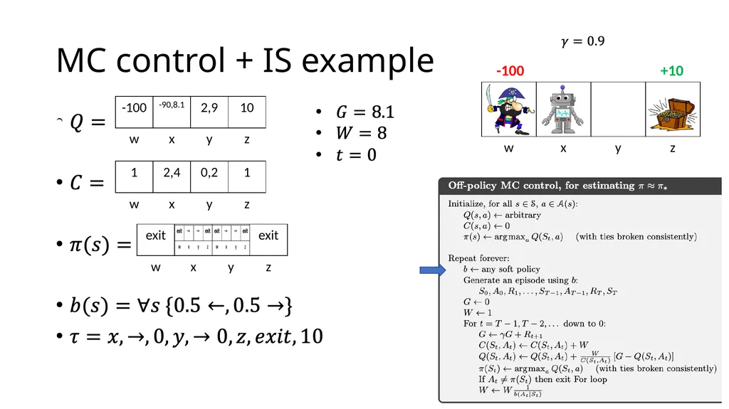
slide35. MC control + importance sampling 35<br>
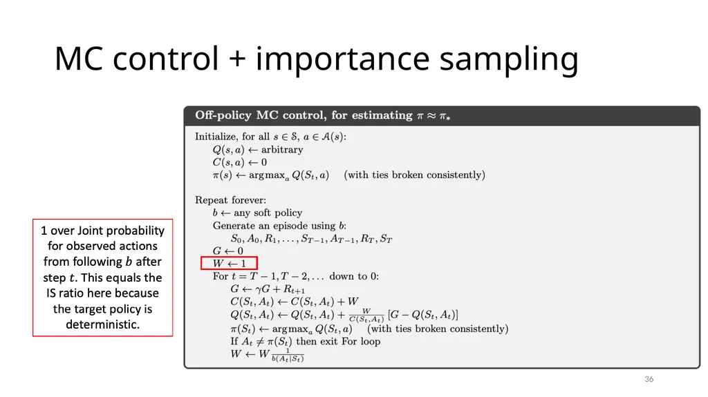
slide36. MC control + importance sampling 36<br>
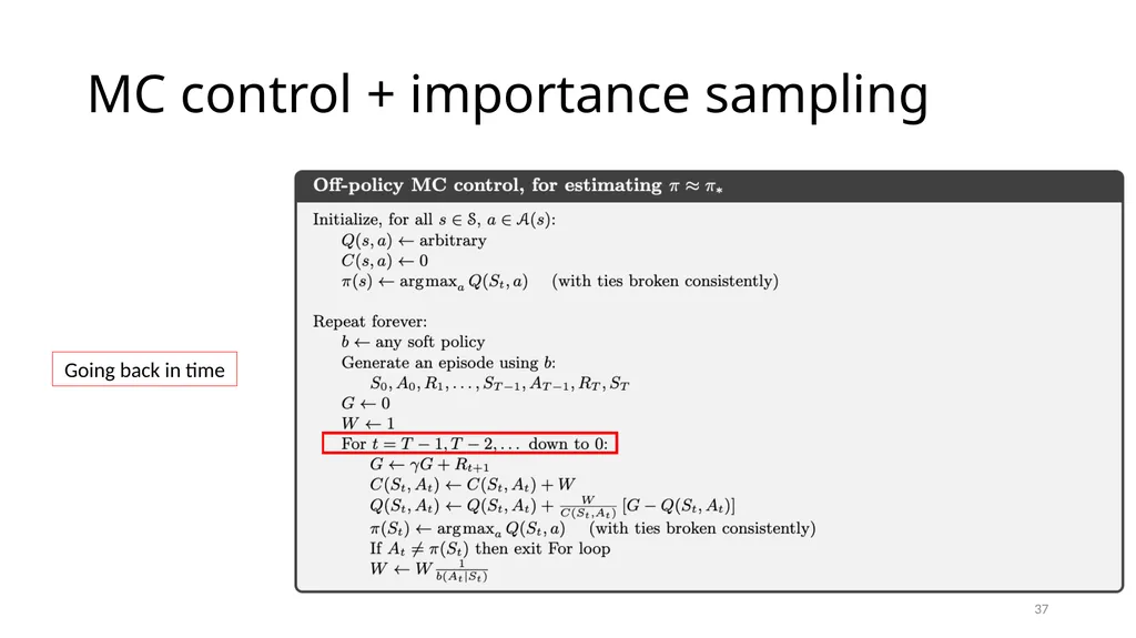
slide37. MC control + importance sampling Going back in time 37<br>
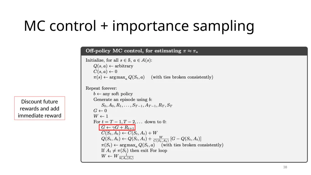
slide38. MC control + importance sampling Discount future rewards and add immediate reward 38<br>
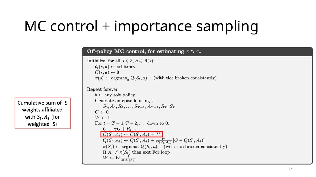
slide39. MC control + importance sampling 39<br>
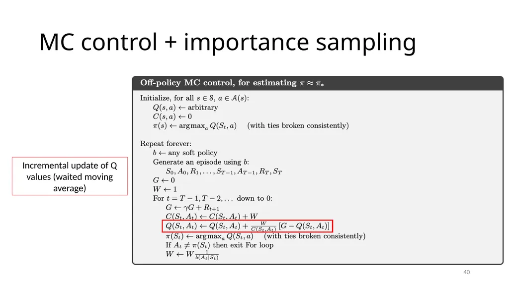
slide40. MC control + importance sampling Incremental update of Q values (waited moving average) 40<br>
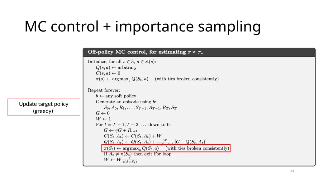
slide41. MC control + importance sampling Update target policy (greedy) 41<br>
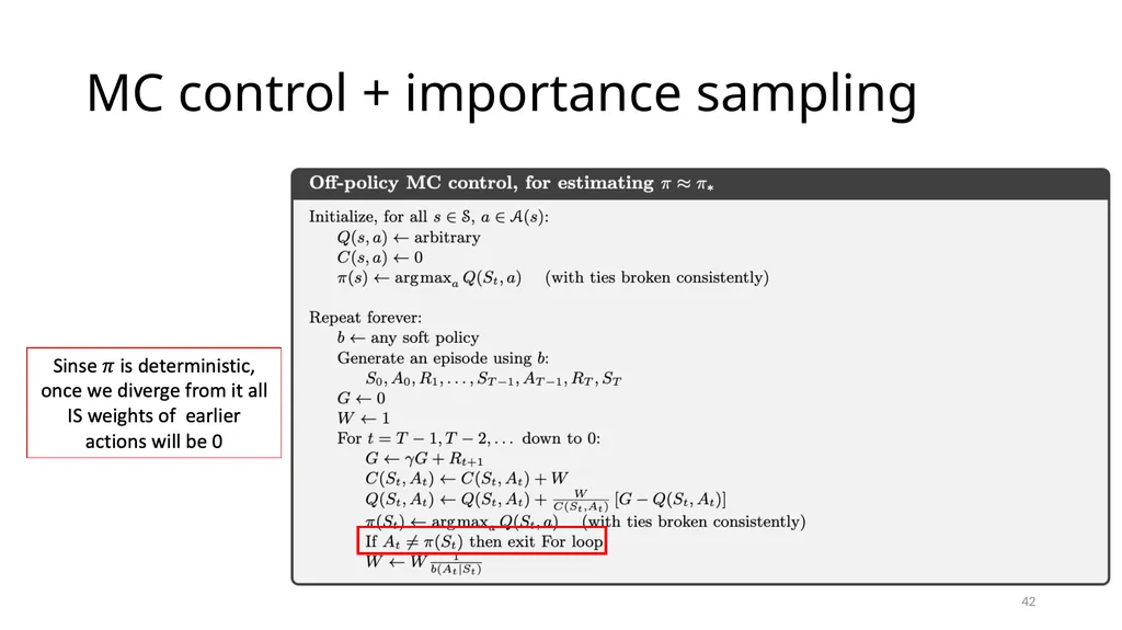
slide42. MC control + importance sampling 42<br>
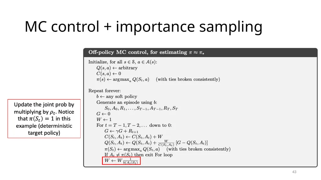
slide43. MC control + importance sampling 43<br>
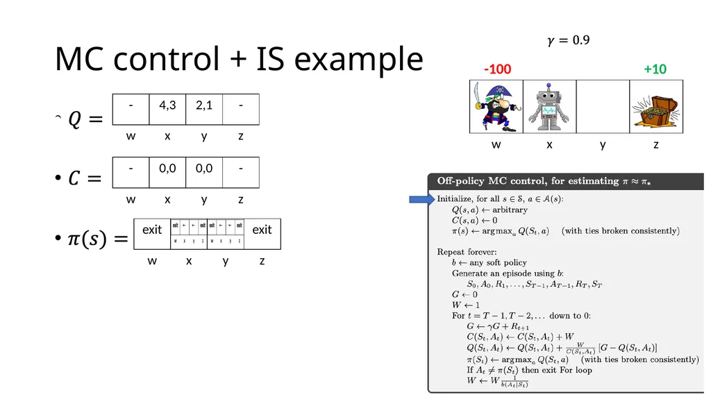
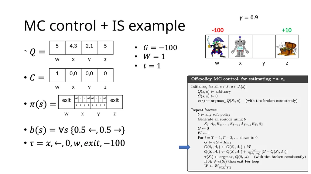
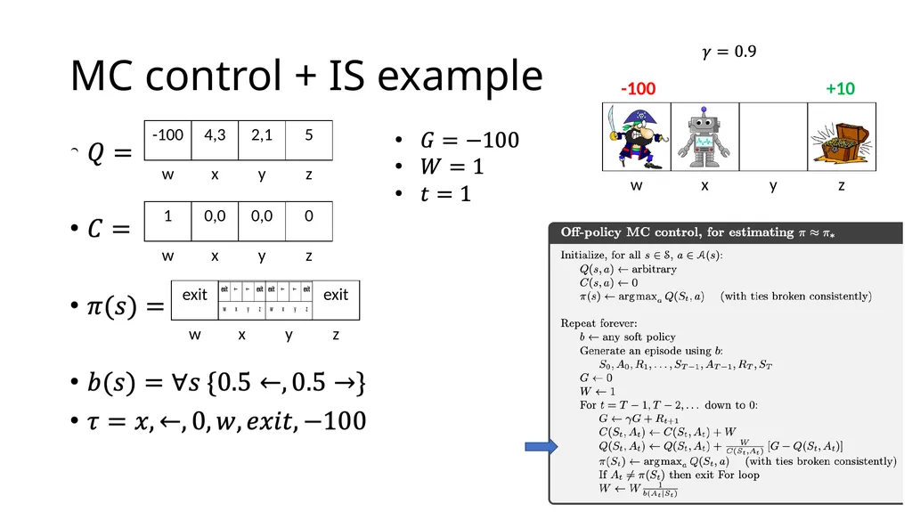
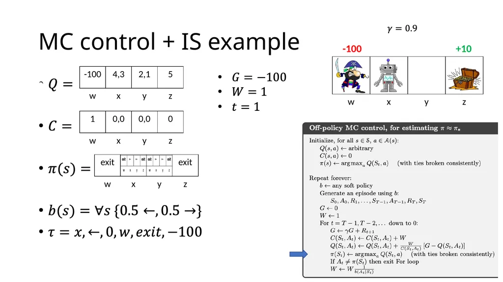
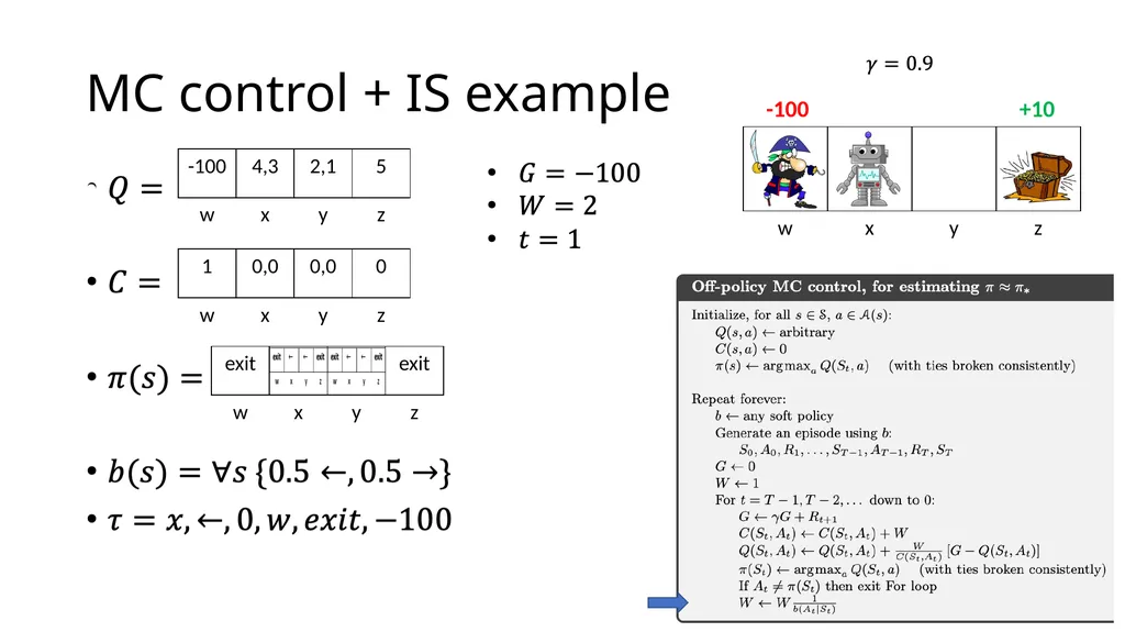
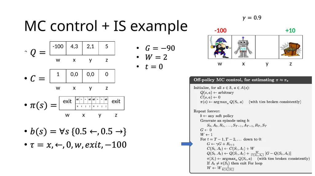
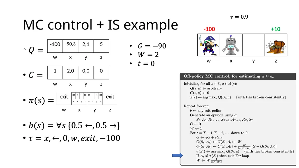
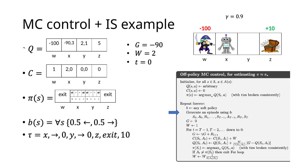
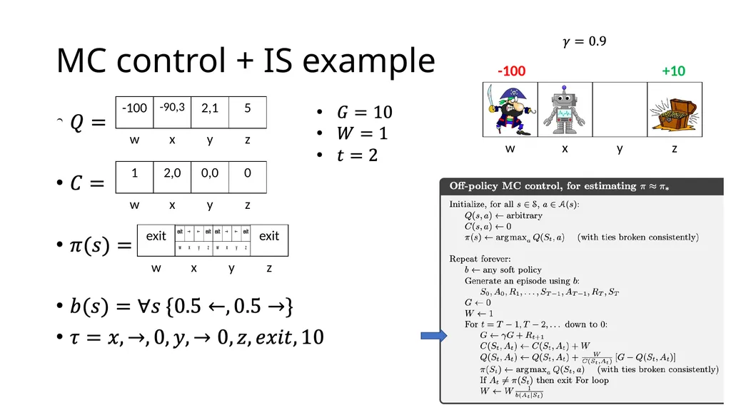
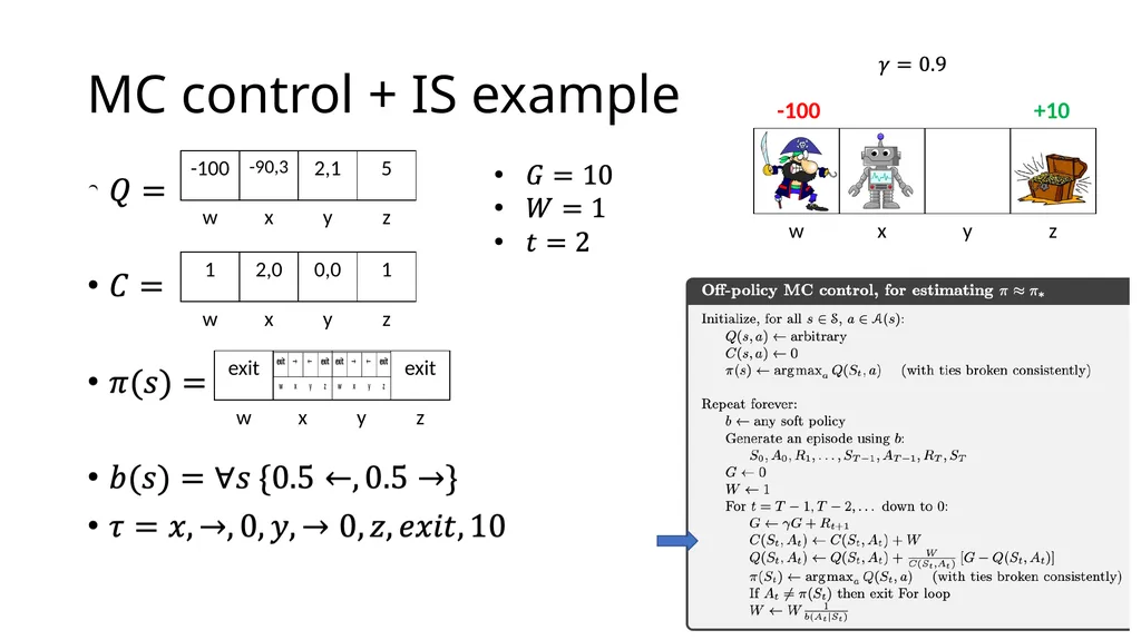
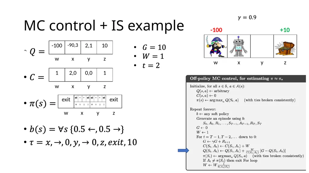
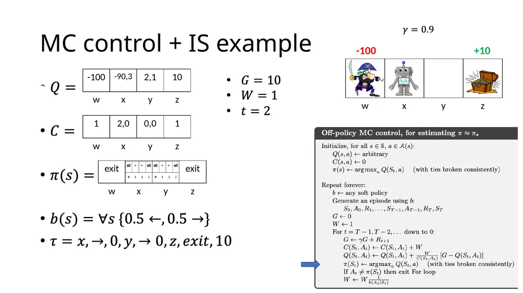
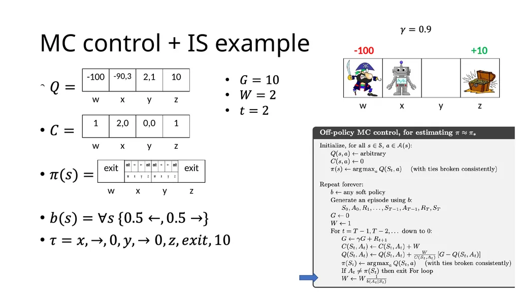
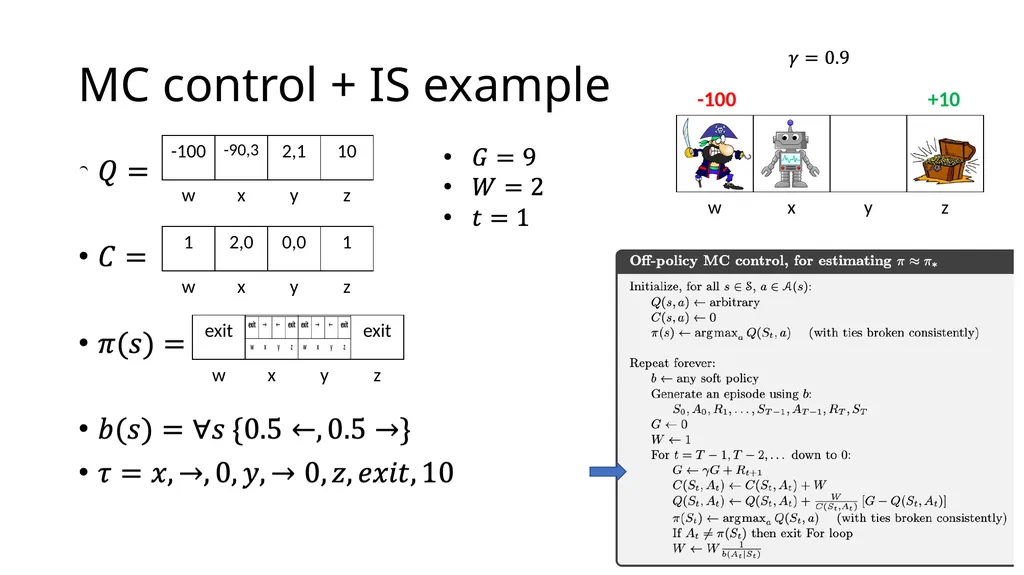
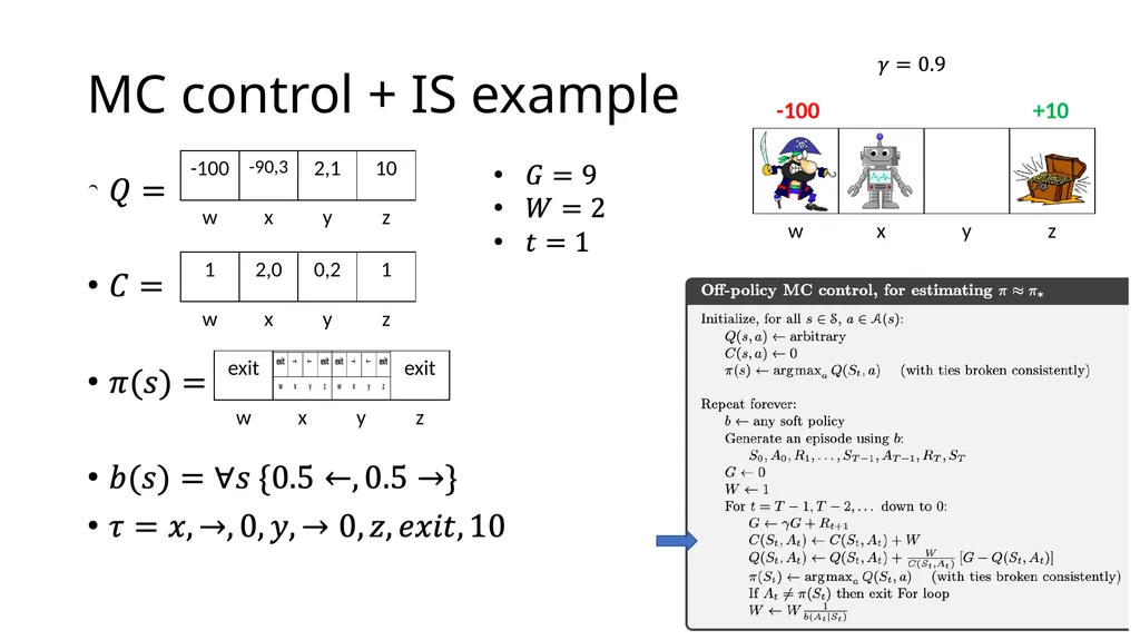
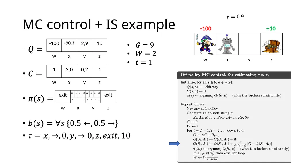
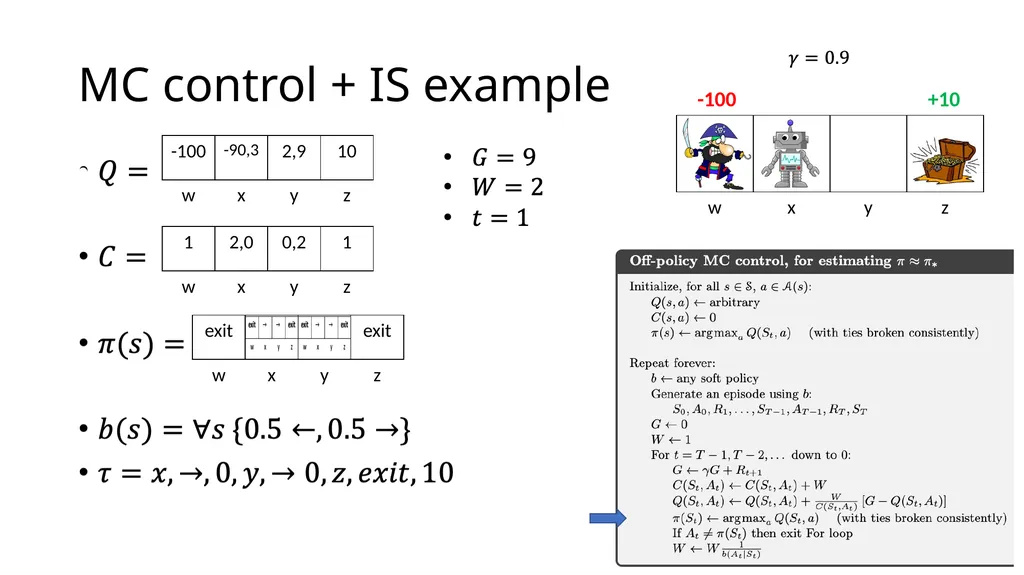
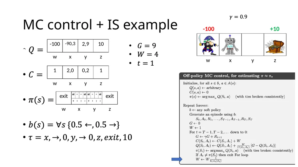
slide44. MC control + IS example +10 -100 44<br>
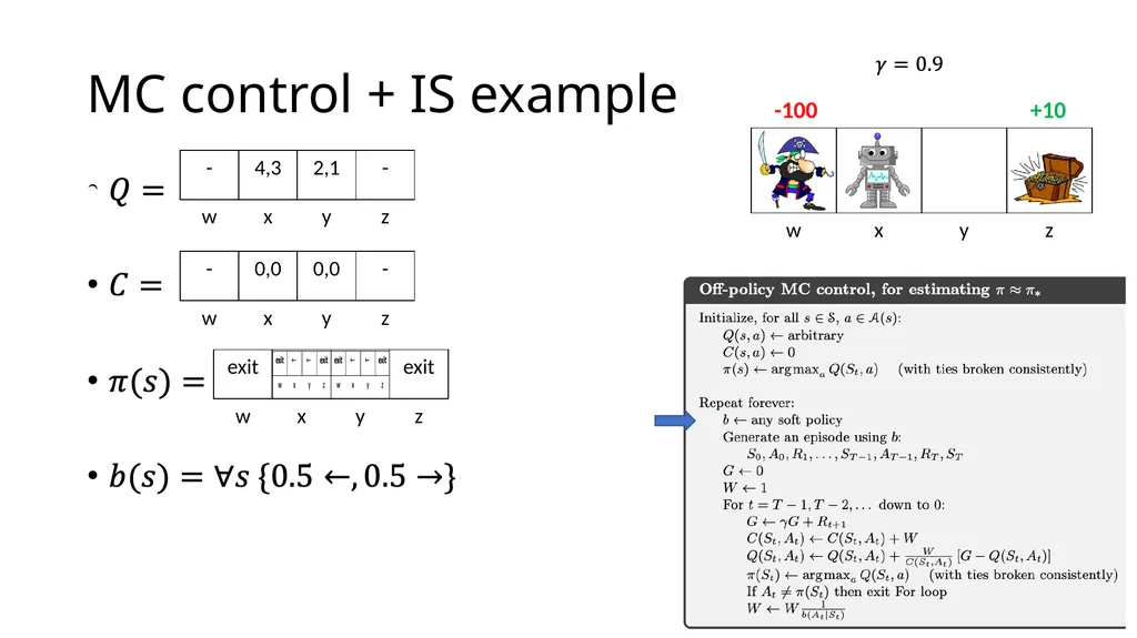
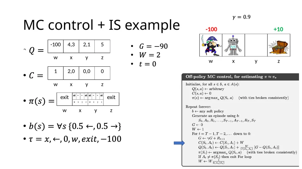
slide45. MC control + IS example +10 -100 45<br>
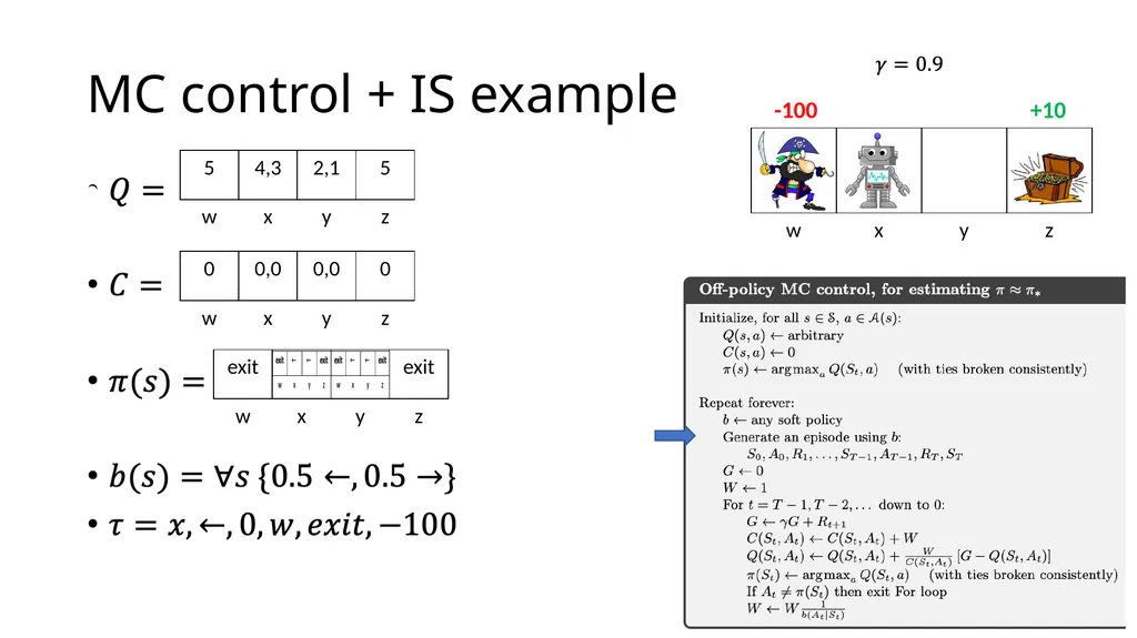
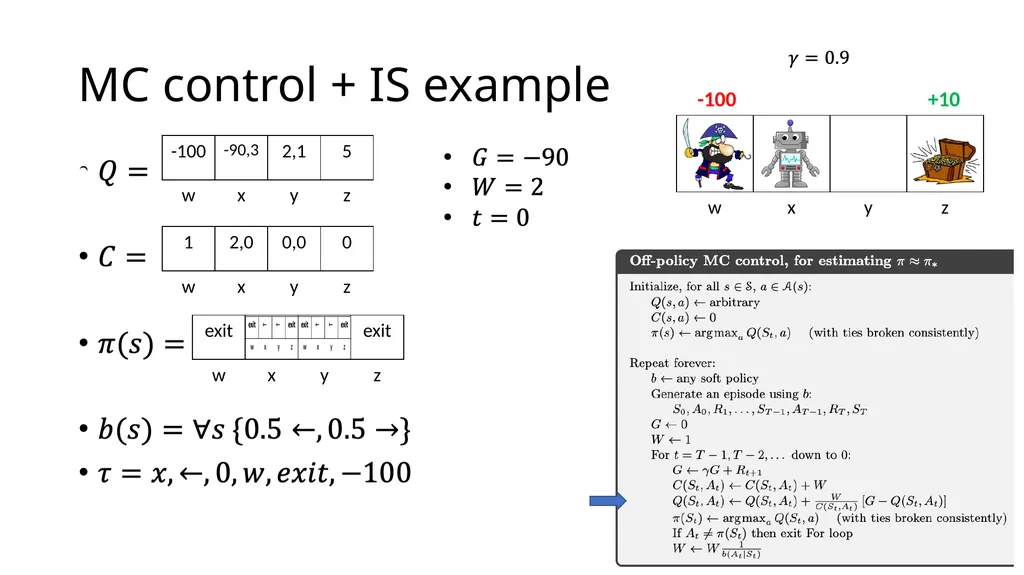
slide46. MC control + IS example +10 -100 46<br>
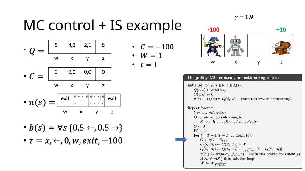
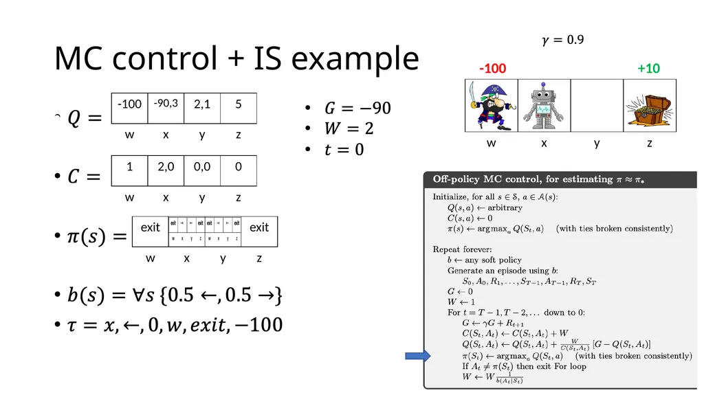
slide47. MC control + IS example +10 -100 47<br>
slide48. MC control + IS example +10 -100 48<br>
slide49. MC control + IS example +10 -100 49<br>
slide50. MC control + IS example +10 -100 50<br>
slide51. MC control + IS example +10 -100 51<br>
slide52. MC control + IS example +10 -100 52<br>
slide53. MC control + IS example +10 -100 53<br>
slide54. MC control + IS example +10 -100 54<br>
slide55. MC control + IS example +10 -100 55<br>
slide56. MC control + IS example +10 -100 56<br>
slide57. MC control + IS example +10 -100 57<br>
slide58. MC control + IS example +10 -100 58<br>
slide59. MC control + IS example +10 -100 59<br>
slide60. MC control + IS example +10 -100 60<br>
slide61. MC control + IS example +10 -100 61<br>
slide62. MC control + IS example +10 -100 62<br>
slide63. MC control + IS example +10 -100 63<br>
slide64. MC control + IS example +10 -100 64<br>
slide65. MC control + IS example +10 -100 65<br>
slide66. MC control + IS example +10 -100 66<br>
slide67. MC control + IS example +10 -100 67<br>
slide68. MC control + IS example +10 -100 68<br>
slide69. MC control + IS example +10 -100 69<br>
slide70. MC control + IS example +10 -100 70<br>
slide71. MC control + IS example +10 -100 71<br>
slide72. MC control + IS example +10 -100 72<br>
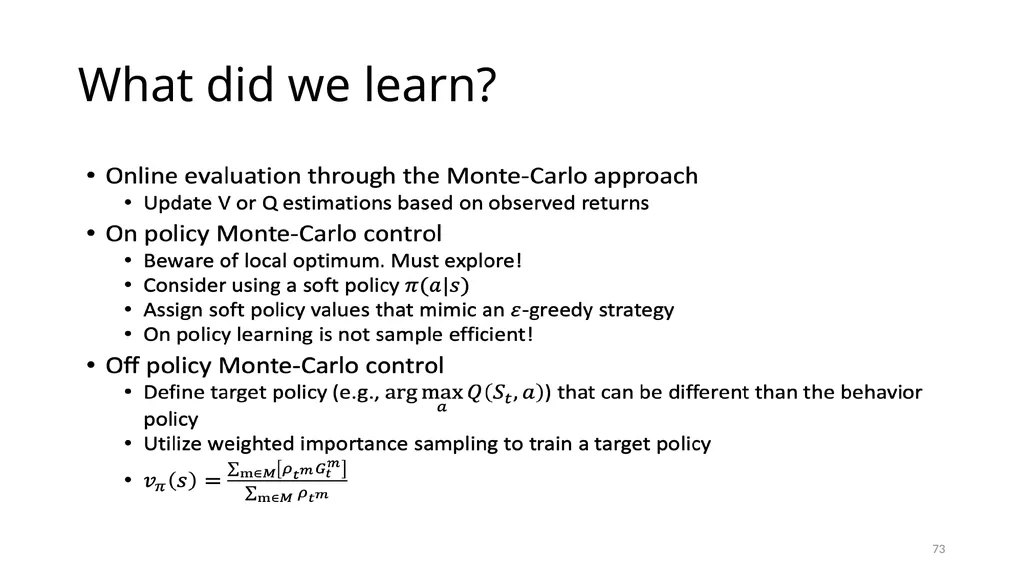
slide73. What did we learn? 73<br>
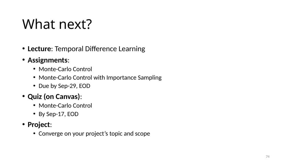
slide74. What next? Lecture: Temporal Difference Learning
Assignments:
Monte-Carlo Control
Monte-Carlo Control with Importance Sampling
Due by Sep-29, EOD
Quiz (on Canvas):
Monte-Carlo Control
By Sep-17, EOD
Project:
Converge on your project’s topic and scope 74<br>
slide2. CSCE-689, Reinforcement Learning Stateless decision process Markov decision process Solving MDPs (offline) Dynamic programming Monte-Carlo Temporal difference Tabular methods Function approximators Policy gradient Deep RL Actor-critic 2<br>
slide3. Reinforcement Learning 3<br>
slide4. Offline vs. Online (RL) Offline Optimization Online Learning 4<br>
slide5. Monte-Carlo Methods Monte Carlo methods are a broad class of computational algorithms that rely on repeated random sampling to obtain numerical results
The underlying concept is to obtain unbiased samples from a complex/unknown distribution through a random process
They are often used in physical and mathematical problems and are most useful when it is difficult or impossible to compute a solution analytically
Weather prediction
Computational biology
Computer graphics
Finance and business
Sport game prediction 5<br>
slide6. Value-based learning via Monte-Carlo r 6<br>
slide7. Example: MC Evaluation Input Policy Assume: = 1 Observed Episodes (Training) Output Values B, east, C, -1
C, east, D, -1
D, exit, , +10 B, east, C, -1
C, east, D, -1
D, exit, , +10 E, north, C, -1
C, east, A, -1
A, exit, , -10 Episode 1 Episode 2 Episode 3 Episode 4 E, north, C, -1
C, east, D, -1
D, exit, , +10 +8 +4 +10 -10 -2 7<br>
slide8. Problems with MC Evaluation What’s good about direct evaluation?
It’s easy to understand
It doesn’t require any knowledge of the model
It converges to the true expected values
What’s bad about it?
It wastes information about transition probabilities
Each state must be learned separately
So, it takes a long time to learn Output Values +8 +4 +10 -10 -2 If B and E both go to C with the same probability, how can their values be different? 8<br>
slide9. Greedy MC +10 -1 +1 9<br>
slide10. Greedy MC +10 -1 +1 10<br>
slide11. Greedy MC +10 -1 +1 We converged on a local optimum! 11<br>
slide12. Must explore! 12<br>
slide13. 13<br>
slide14. MC control - example +10 -100 14<br>
slide15. MC control - example +10 -100 15<br>
slide16. MC control - example +10 -100 16<br>
slide17. MC control - example +10 -100 17<br>
slide18. MC control - example +10 -100 18<br>
slide19. MC control - example +10 -100 19<br>
slide20. MC control - example +10 -100 20<br>
slide21. MC control - example +10 -100 21<br>
slide22. MC control - example +10 -100 22<br>
slide23. MC control - example +10 -100 23<br>
slide24. On-policy learning +10 -1 +1 24 Estimation True value<br>
slide25. Off-policy learning 25<br>
slide26. Off-policy learning conditions 26<br>
slide27. Trajectory probability 27<br>
slide28. Importance sampling YES! 28<br>
slide29. Importance sampling 29<br>
slide30. Importance sampling: proof 30<br>
slide31. Importance sampling: proof 31 Importance ratio<br>
slide32. (ordinary) Importance sampling - example +10 -1 +1 32<br>
slide33. Weighted importance sampling +10 -1 +1 Ordinary Importance sampling is unbiased while the weighted version is biased (initially). Ordinary Importance sampling results in high variance while the weighted version has a bounded variance Trick: normalize by the sum of importance ratios 33<br>
slide34. Ordinary vs weighted importance sampling Estimating a black-jack state
Target policy: hit on 19 or below
Behavior policy: random (uniform)
Both approaches converge to the true value
weighted importance sampling is much better initially 34<br>
slide35. MC control + importance sampling 35<br>
slide36. MC control + importance sampling 36<br>
slide37. MC control + importance sampling Going back in time 37<br>
slide38. MC control + importance sampling Discount future rewards and add immediate reward 38<br>
slide39. MC control + importance sampling 39<br>
slide40. MC control + importance sampling Incremental update of Q values (waited moving average) 40<br>
slide41. MC control + importance sampling Update target policy (greedy) 41<br>
slide42. MC control + importance sampling 42<br>
slide43. MC control + importance sampling 43<br>
slide44. MC control + IS example +10 -100 44<br>
slide45. MC control + IS example +10 -100 45<br>
slide46. MC control + IS example +10 -100 46<br>
slide47. MC control + IS example +10 -100 47<br>
slide48. MC control + IS example +10 -100 48<br>
slide49. MC control + IS example +10 -100 49<br>
slide50. MC control + IS example +10 -100 50<br>
slide51. MC control + IS example +10 -100 51<br>
slide52. MC control + IS example +10 -100 52<br>
slide53. MC control + IS example +10 -100 53<br>
slide54. MC control + IS example +10 -100 54<br>
slide55. MC control + IS example +10 -100 55<br>
slide56. MC control + IS example +10 -100 56<br>
slide57. MC control + IS example +10 -100 57<br>
slide58. MC control + IS example +10 -100 58<br>
slide59. MC control + IS example +10 -100 59<br>
slide60. MC control + IS example +10 -100 60<br>
slide61. MC control + IS example +10 -100 61<br>
slide62. MC control + IS example +10 -100 62<br>
slide63. MC control + IS example +10 -100 63<br>
slide64. MC control + IS example +10 -100 64<br>
slide65. MC control + IS example +10 -100 65<br>
slide66. MC control + IS example +10 -100 66<br>
slide67. MC control + IS example +10 -100 67<br>
slide68. MC control + IS example +10 -100 68<br>
slide69. MC control + IS example +10 -100 69<br>
slide70. MC control + IS example +10 -100 70<br>
slide71. MC control + IS example +10 -100 71<br>
slide72. MC control + IS example +10 -100 72<br>
slide73. What did we learn? 73<br>
slide74. What next? Lecture: Temporal Difference Learning
Assignments:
Monte-Carlo Control
Monte-Carlo Control with Importance Sampling
Due by Sep-29, EOD
Quiz (on Canvas):
Monte-Carlo Control
By Sep-17, EOD
Project:
Converge on your project’s topic and scope 74<br>