
CSE 5403: Stochastic Process Cr. 3.00 Course
Description: CSE 5403: Stochastic Process Cr. 3.00 Course Leaner: 2nd semester of MS 2015-16 Course Teacher: A H M Kamal Normal Distribution: In probability theory, the normal (or Gaussian or Gauss or Laplace-Gauss) distribution is a very common
Related Topics
Download Presentation
"CSE 5403: Stochastic Process Cr. 3.00 Course" is the property of its rightful owner. Permission is granted to download and print the materials on this website for personal, non-commercial use only, and to display it on your personal computer provided you do not modify the materials and that you retain all copyright notices contained in the materials. By downloading content from our website, you accept the terms of this agreement.
Presentation Transcript
slide1. CSE 5403: Stochastic Process Cr. 3.00 Course Leaner: 2nd semester of MS 2015-16 Course Teacher: A H M Kamal<br>
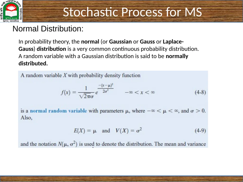
slide2. Normal Distribution: In probability theory, the normal (or Gaussian or Gauss or Laplace-Gauss) distribution is a very common continuous probability distribution.
A random variable with a Gaussian distribution is said to be normally distributed.<br>
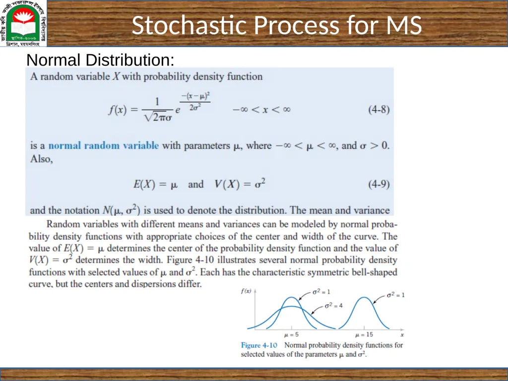
slide3. Normal Distribution:<br>
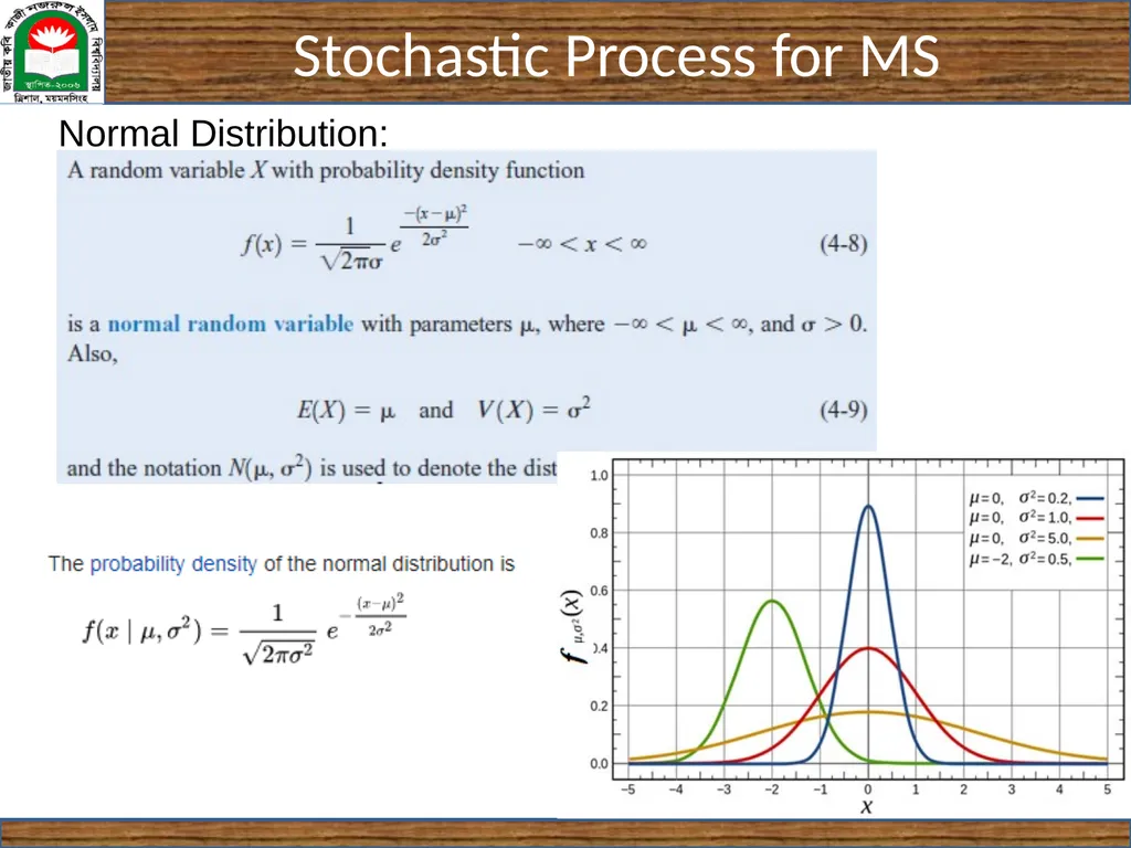
slide4. Normal Distribution:<br>
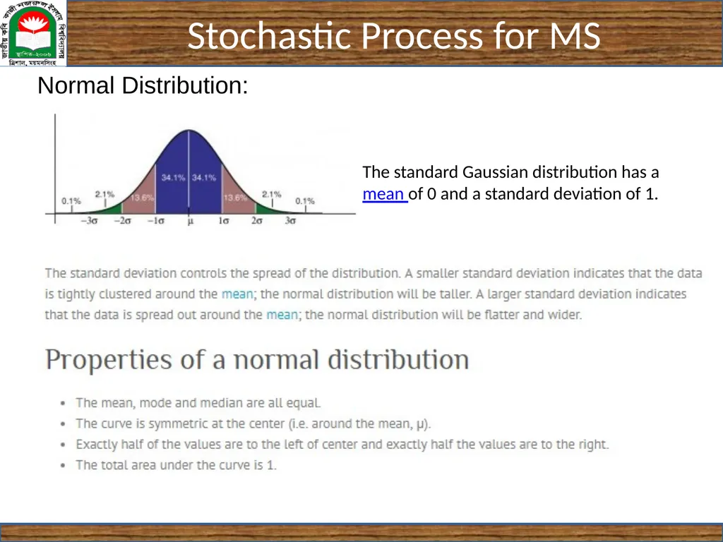
slide5. Normal Distribution: The standard Gaussian distribution has a mean of 0 and a standard deviation of 1.<br>
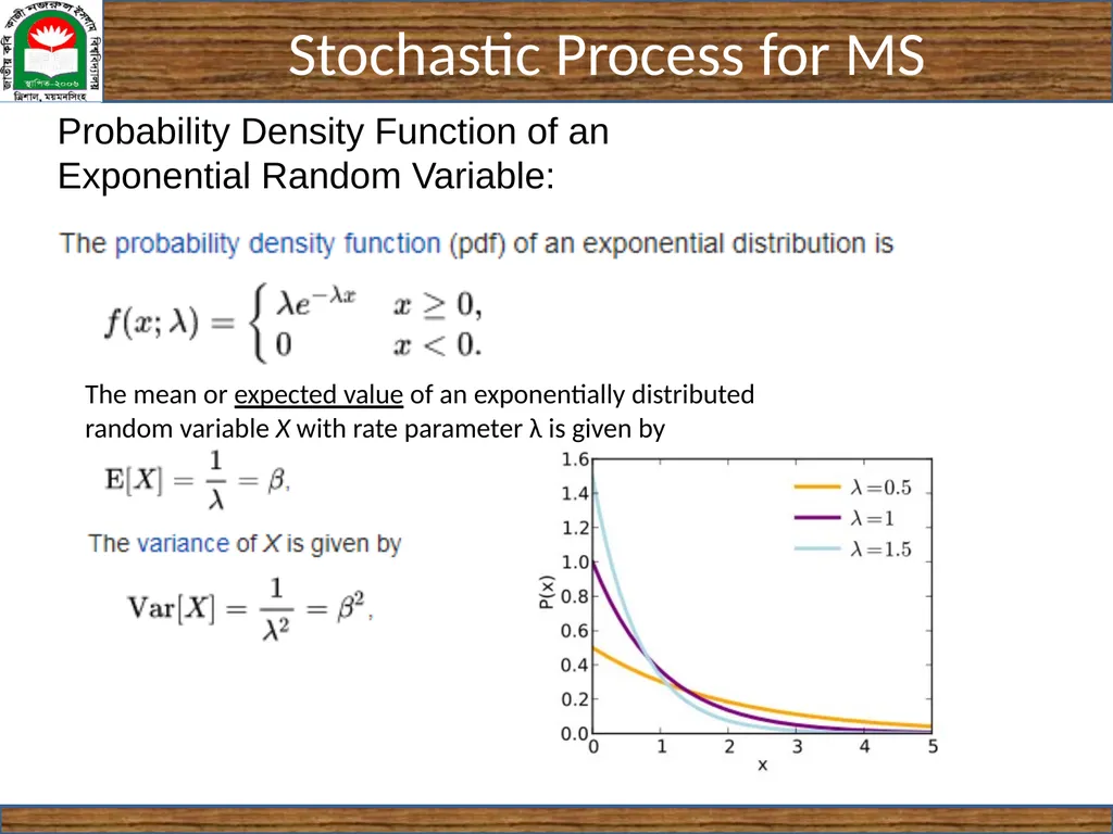
slide6. Probability Density Function of an Exponential Random Variable: The mean or expected value of an exponentially distributed random variable X with rate parameter λ is given by<br>
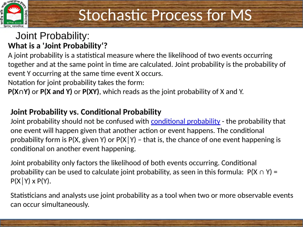
slide7. Joint Probability: What is a 'Joint Probability‘?
A joint probability is a statistical measure where the likelihood of two events occurring together and at the same point in time are calculated. Joint probability is the probability of event Y occurring at the same time event X occurs.
Notation for joint probability takes the form:
P(X∩Y) or P(X and Y) or P(XY), which reads as the joint probability of X and Y. Joint Probability vs. Conditional Probability
Joint probability should not be confused with conditional probability - the probability that one event will happen given that another action or event happens. The conditional probability form is P(X, given Y) or P(X│Y) – that is, the chance of one event happening is conditional on another event happening. Joint probability only factors the likelihood of both events occurring. Conditional probability can be used to calculate joint probability, as seen in this formula: P(X ∩ Y) = P(X│Y) x P(Y). Statisticians and analysts use joint probability as a tool when two or more observable events can occur simultaneously.<br>
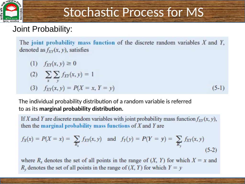
slide8. Joint Probability: The individual probability distribution of a random variable is referred
to as its marginal probability distribution.<br>
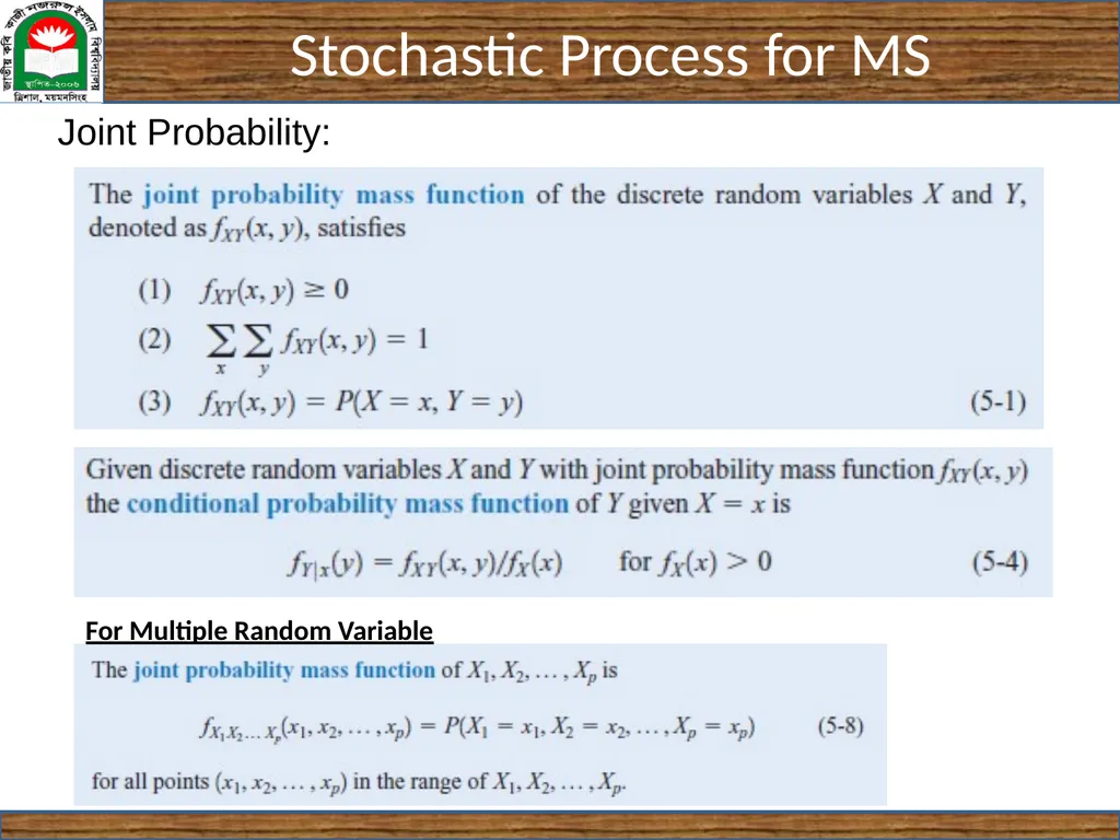
slide9. Joint Probability: For Multiple Random Variable<br>
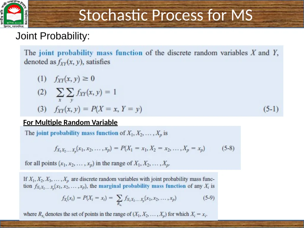
slide10. Joint Probability: For Multiple Random Variable<br>
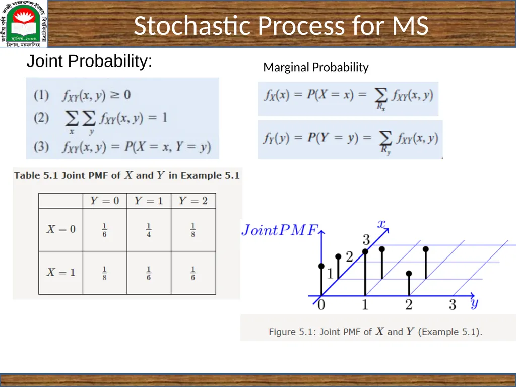
slide11. Joint Probability: Marginal Probability<br>
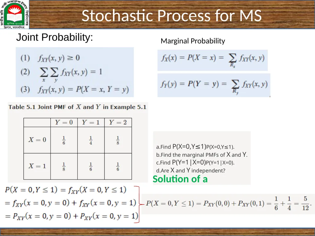
slide12. Joint Probability: Find P(X=0,Y≤1)P(X=0,Y≤1).
Find the marginal PMFs of X and Y.
Find P(Y=1|X=0)P(Y=1|X=0).
Are X and Y independent? Marginal Probability Solution of a<br>
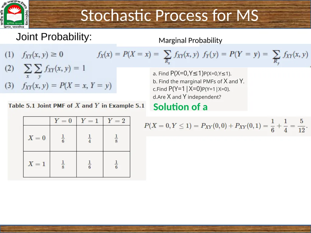
slide13. Joint Probability: a. Find P(X=0,Y≤1)P(X=0,Y≤1).
b. Find the marginal PMFs of X and Y.
Find P(Y=1|X=0)P(Y=1|X=0).
Are X and Y independent? Marginal Probability Solution of a<br>
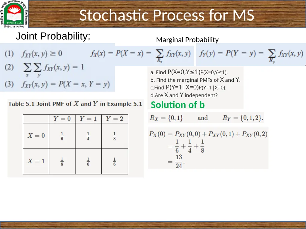
slide14. Joint Probability: a. Find P(X=0,Y≤1)P(X=0,Y≤1).
b. Find the marginal PMFs of X and Y.
Find P(Y=1|X=0)P(Y=1|X=0).
Are X and Y independent? Marginal Probability Solution of b<br>
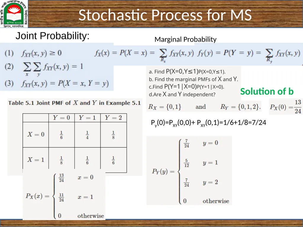
slide15. Joint Probability: a. Find P(X=0,Y≤1)P(X=0,Y≤1).
b. Find the marginal PMFs of X and Y.
Find P(Y=1|X=0)P(Y=1|X=0).
Are X and Y independent? Marginal Probability Py(0)=PXY(0,0)+ PXY(0,1)=1/6+1/8=7/24 Solution of b<br>
slide16. Joint Probability: a. Find P(X=0,Y≤1)P(X=0,Y≤1).
b. Find the marginal PMFs of X and Y.
Find P(Y=1|X=0)P(Y=1|X=0).
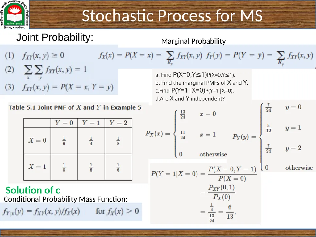
Are X and Y independent? Marginal Probability Conditional Probability Mass Function: Solution of c<br>
slide17. Joint Probability: a. Find P(X=0,Y≤1)P(X=0,Y≤1).
b. Find the marginal PMFs of X and Y.
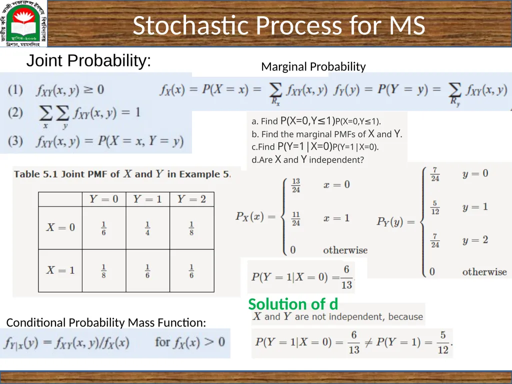
Find P(Y=1|X=0)P(Y=1|X=0).
Are X and Y independent? Marginal Probability Conditional Probability Mass Function: Solution of d<br>
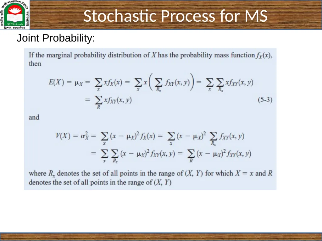
slide18. Joint Probability:<br>
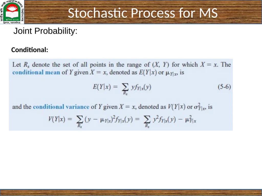
slide19. Joint Probability: Conditional:<br>
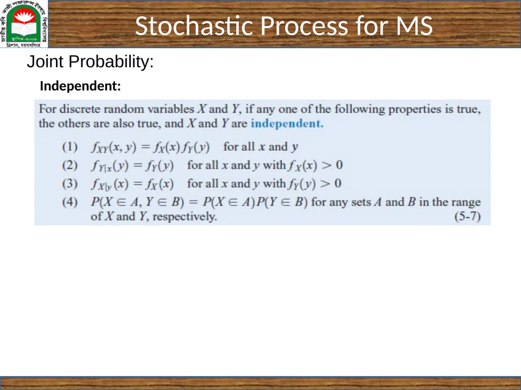
slide20. Joint Probability: Independent:<br>
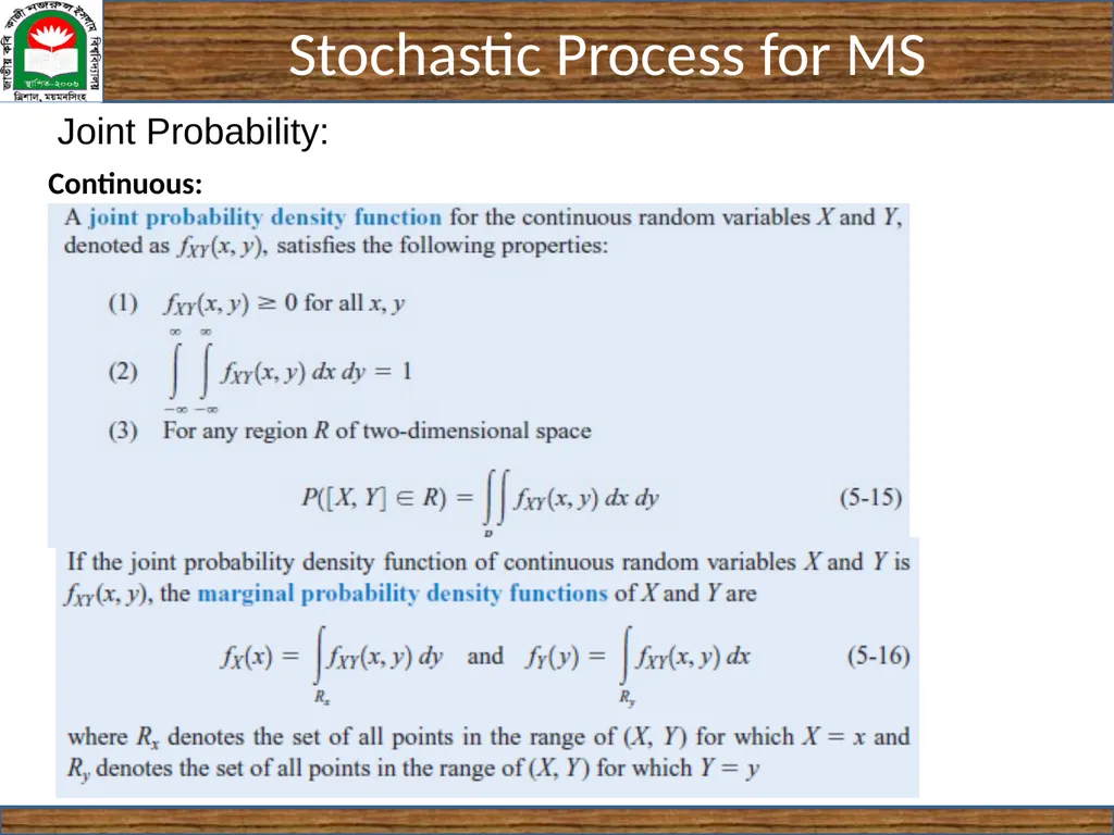
slide21. Joint Probability: Continuous:<br>
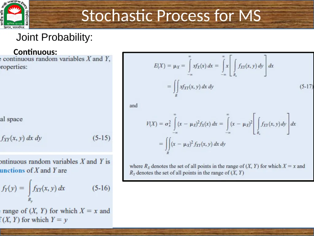
slide22. Joint Probability: Continuous:<br>
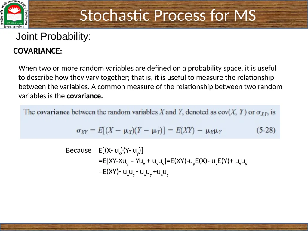
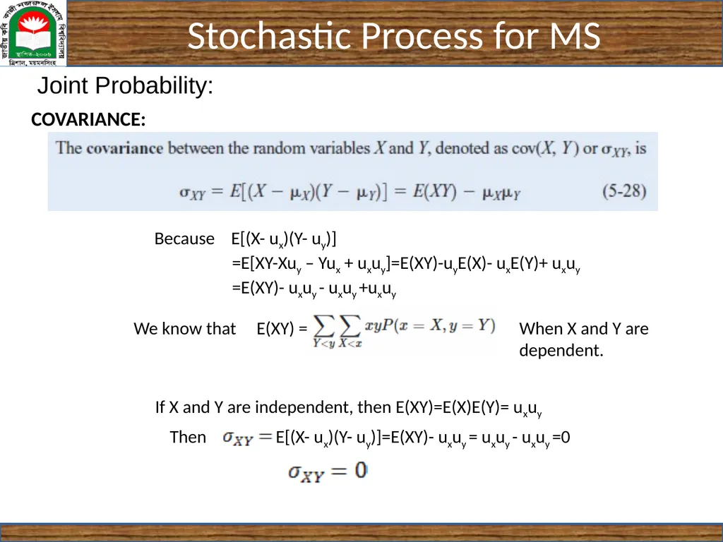
slide23. Joint Probability: COVARIANCE: When two or more random variables are defined on a probability space, it is useful to describe how they vary together; that is, it is useful to measure the relationship between the variables. A common measure of the relationship between two random variables is the covariance. Because E[(X- ux)(Y- uy)]
=E[XY-Xuy – Yux + uxuy]=E(XY)-uyE(X)- uxE(Y)+ uxuy
=E(XY)- uxuy - uxuy +uxuy<br>
slide24. Joint Probability: COVARIANCE: Because E[(X- ux)(Y- uy)]
=E[XY-Xuy – Yux + uxuy]=E(XY)-uyE(X)- uxE(Y)+ uxuy
=E(XY)- uxuy - uxuy +uxuy<br>
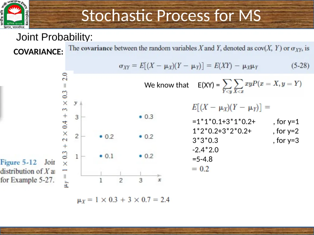
slide25. Joint Probability: COVARIANCE:<br>
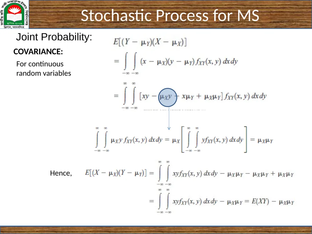
slide26. Joint Probability: COVARIANCE: For continuous
random variables<br>
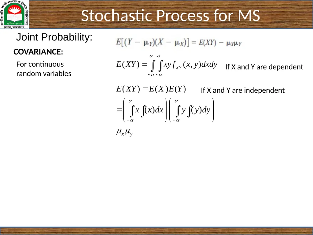
slide27. Joint Probability: COVARIANCE: For continuous
random variables<br>
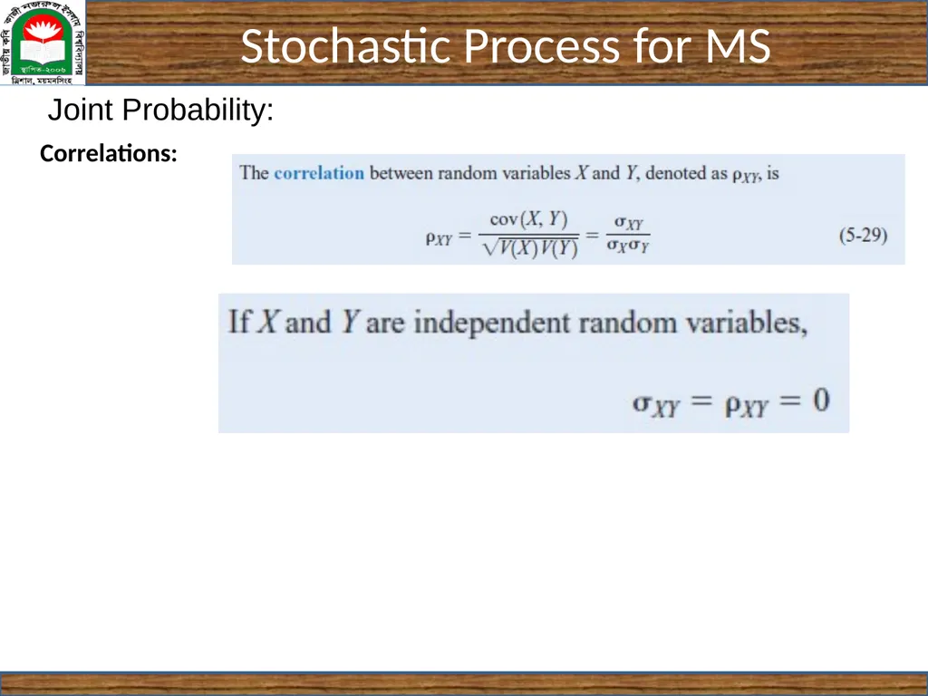
slide28. Joint Probability: Correlations:<br>
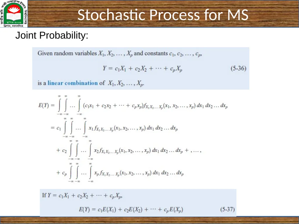
slide29. Joint Probability:<br>
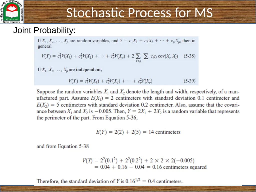
slide30. Joint Probability:<br>
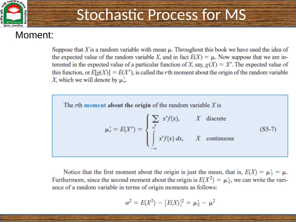
slide31. Moment:<br>
slide2. Normal Distribution: In probability theory, the normal (or Gaussian or Gauss or Laplace-Gauss) distribution is a very common continuous probability distribution.
A random variable with a Gaussian distribution is said to be normally distributed.<br>
slide3. Normal Distribution:<br>
slide4. Normal Distribution:<br>
slide5. Normal Distribution: The standard Gaussian distribution has a mean of 0 and a standard deviation of 1.<br>
slide6. Probability Density Function of an Exponential Random Variable: The mean or expected value of an exponentially distributed random variable X with rate parameter λ is given by<br>
slide7. Joint Probability: What is a 'Joint Probability‘?
A joint probability is a statistical measure where the likelihood of two events occurring together and at the same point in time are calculated. Joint probability is the probability of event Y occurring at the same time event X occurs.
Notation for joint probability takes the form:
P(X∩Y) or P(X and Y) or P(XY), which reads as the joint probability of X and Y. Joint Probability vs. Conditional Probability
Joint probability should not be confused with conditional probability - the probability that one event will happen given that another action or event happens. The conditional probability form is P(X, given Y) or P(X│Y) – that is, the chance of one event happening is conditional on another event happening. Joint probability only factors the likelihood of both events occurring. Conditional probability can be used to calculate joint probability, as seen in this formula: P(X ∩ Y) = P(X│Y) x P(Y). Statisticians and analysts use joint probability as a tool when two or more observable events can occur simultaneously.<br>
slide8. Joint Probability: The individual probability distribution of a random variable is referred
to as its marginal probability distribution.<br>
slide9. Joint Probability: For Multiple Random Variable<br>
slide10. Joint Probability: For Multiple Random Variable<br>
slide11. Joint Probability: Marginal Probability<br>
slide12. Joint Probability: Find P(X=0,Y≤1)P(X=0,Y≤1).
Find the marginal PMFs of X and Y.
Find P(Y=1|X=0)P(Y=1|X=0).
Are X and Y independent? Marginal Probability Solution of a<br>
slide13. Joint Probability: a. Find P(X=0,Y≤1)P(X=0,Y≤1).
b. Find the marginal PMFs of X and Y.
Find P(Y=1|X=0)P(Y=1|X=0).
Are X and Y independent? Marginal Probability Solution of a<br>
slide14. Joint Probability: a. Find P(X=0,Y≤1)P(X=0,Y≤1).
b. Find the marginal PMFs of X and Y.
Find P(Y=1|X=0)P(Y=1|X=0).
Are X and Y independent? Marginal Probability Solution of b<br>
slide15. Joint Probability: a. Find P(X=0,Y≤1)P(X=0,Y≤1).
b. Find the marginal PMFs of X and Y.
Find P(Y=1|X=0)P(Y=1|X=0).
Are X and Y independent? Marginal Probability Py(0)=PXY(0,0)+ PXY(0,1)=1/6+1/8=7/24 Solution of b<br>
slide16. Joint Probability: a. Find P(X=0,Y≤1)P(X=0,Y≤1).
b. Find the marginal PMFs of X and Y.
Find P(Y=1|X=0)P(Y=1|X=0).
Are X and Y independent? Marginal Probability Conditional Probability Mass Function: Solution of c<br>
slide17. Joint Probability: a. Find P(X=0,Y≤1)P(X=0,Y≤1).
b. Find the marginal PMFs of X and Y.
Find P(Y=1|X=0)P(Y=1|X=0).
Are X and Y independent? Marginal Probability Conditional Probability Mass Function: Solution of d<br>
slide18. Joint Probability:<br>
slide19. Joint Probability: Conditional:<br>
slide20. Joint Probability: Independent:<br>
slide21. Joint Probability: Continuous:<br>
slide22. Joint Probability: Continuous:<br>
slide23. Joint Probability: COVARIANCE: When two or more random variables are defined on a probability space, it is useful to describe how they vary together; that is, it is useful to measure the relationship between the variables. A common measure of the relationship between two random variables is the covariance. Because E[(X- ux)(Y- uy)]
=E[XY-Xuy – Yux + uxuy]=E(XY)-uyE(X)- uxE(Y)+ uxuy
=E(XY)- uxuy - uxuy +uxuy<br>
slide24. Joint Probability: COVARIANCE: Because E[(X- ux)(Y- uy)]
=E[XY-Xuy – Yux + uxuy]=E(XY)-uyE(X)- uxE(Y)+ uxuy
=E(XY)- uxuy - uxuy +uxuy<br>
slide25. Joint Probability: COVARIANCE:<br>
slide26. Joint Probability: COVARIANCE: For continuous
random variables<br>
slide27. Joint Probability: COVARIANCE: For continuous
random variables<br>
slide28. Joint Probability: Correlations:<br>
slide29. Joint Probability:<br>
slide30. Joint Probability:<br>
slide31. Moment:<br>