
Data Mining Classification: Basic Concepts and
CS
Published · 59 slides · 0 views
1 / 1
Description
Data Mining Classification: Basic Concepts and Techniques Lecture Notes for Chapter 3 Introduction to Data Mining, 2nd Edition by Tan, Steinbach, Karpatne, Kumar 212021 Introduction to Data Mining, 2nd Edition 1 Classification: Definition
Related Topics
Share
Embed code
Download this presentation From Below
"Data Mining Classification: Basic Concepts and" is the property of its rightful owner. Permission is granted to download and print the materials on this website for personal, non-commercial use only, and to display it on your personal computer provided you do not modify the materials and that you retain all copyright notices contained in the materials. By downloading content from our website, you accept the terms of this agreement.
Presentation Transcript
01
Data Mining
Classification: Basic Concepts and Techniques Lecture Notes for Chapter 3
Introduction to Data Mining, 2nd Edition
by
Tan, Steinbach, Karpatne, Kumar 2/1/2021 Introduction to Data Mining, 2nd Edition 1<br>
Introduction to Data Mining, 2nd Edition
by
Tan, Steinbach, Karpatne, Kumar 2/1/2021 Introduction to Data Mining, 2nd Edition 1<br>
02
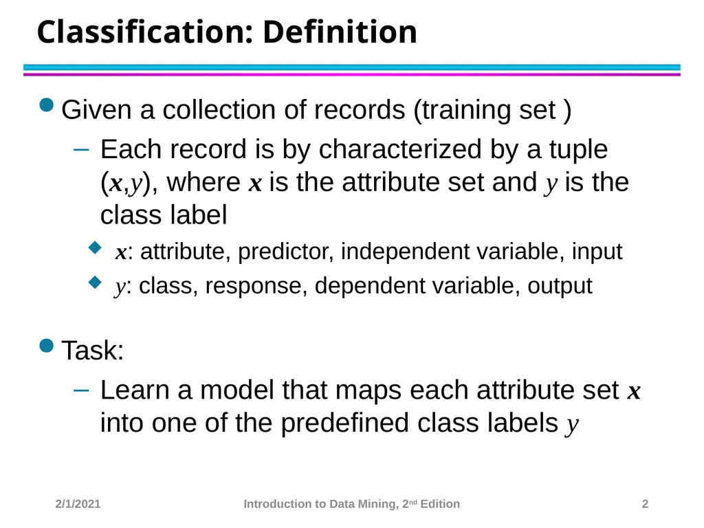
Classification: Definition Given a collection of records (training set )
Each record is by characterized by a tuple (x,y), where x is the attribute set and y is the class label
x: attribute, predictor, independent variable, input
y: class, response, dependent variable, output
Task:
Learn a model that maps each attribute set x into one of the predefined class labels y 2/1/2021 Introduction to Data Mining, 2nd Edition 2<br>
Each record is by characterized by a tuple (x,y), where x is the attribute set and y is the class label
x: attribute, predictor, independent variable, input
y: class, response, dependent variable, output
Task:
Learn a model that maps each attribute set x into one of the predefined class labels y 2/1/2021 Introduction to Data Mining, 2nd Edition 2<br>
03
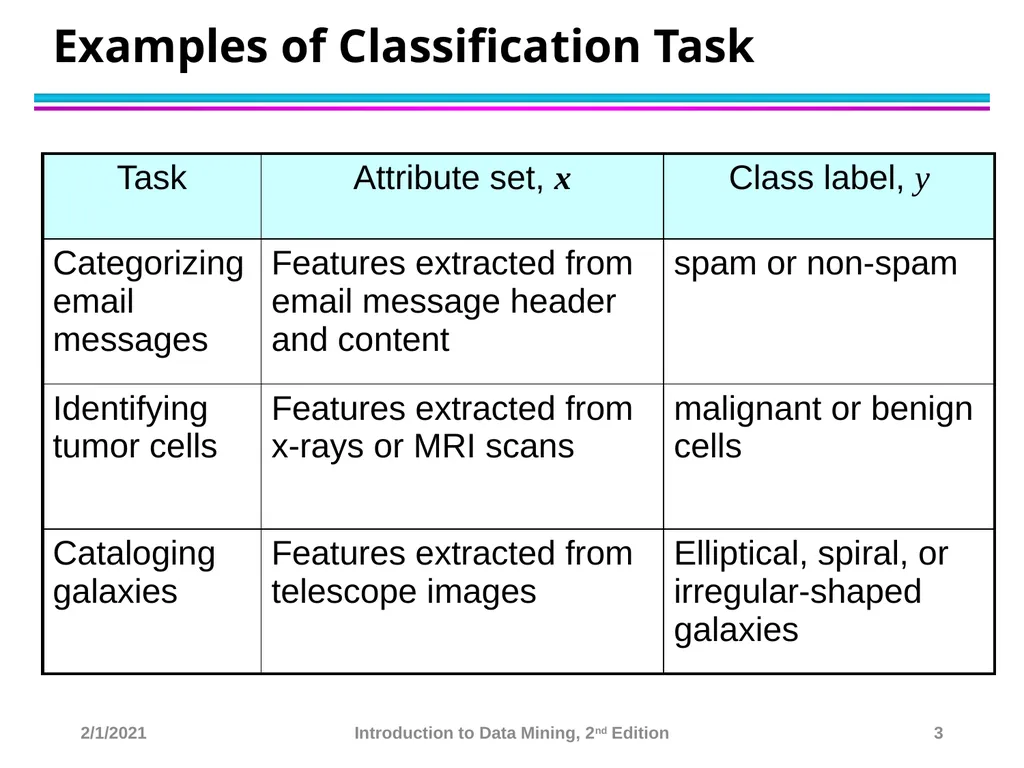
Examples of Classification Task 2/1/2021 Introduction to Data Mining, 2nd Edition 3<br>
04
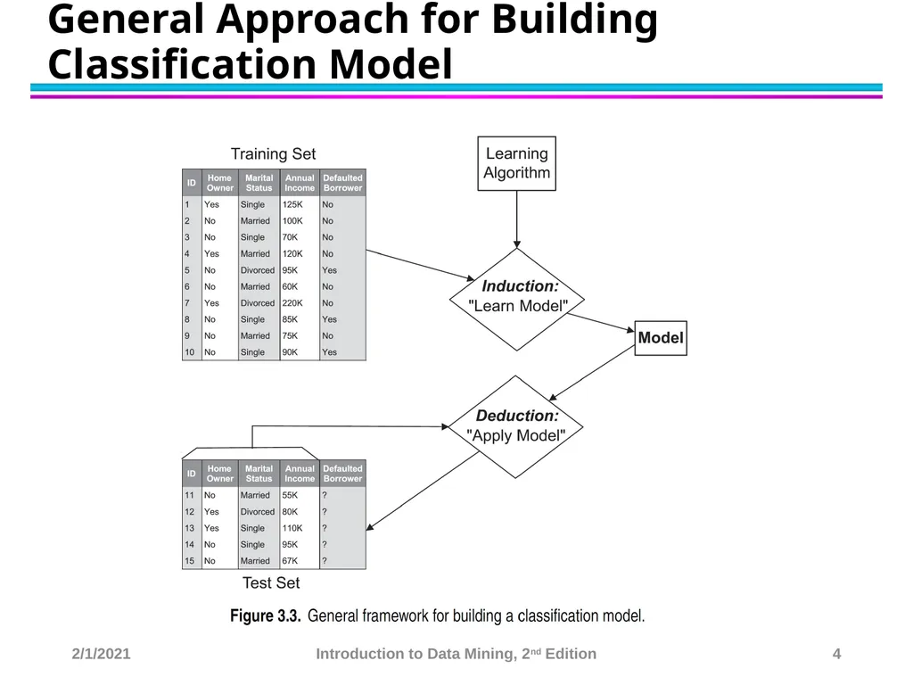
General Approach for Building Classification Model 2/1/2021 Introduction to Data Mining, 2nd Edition 4<br>
05
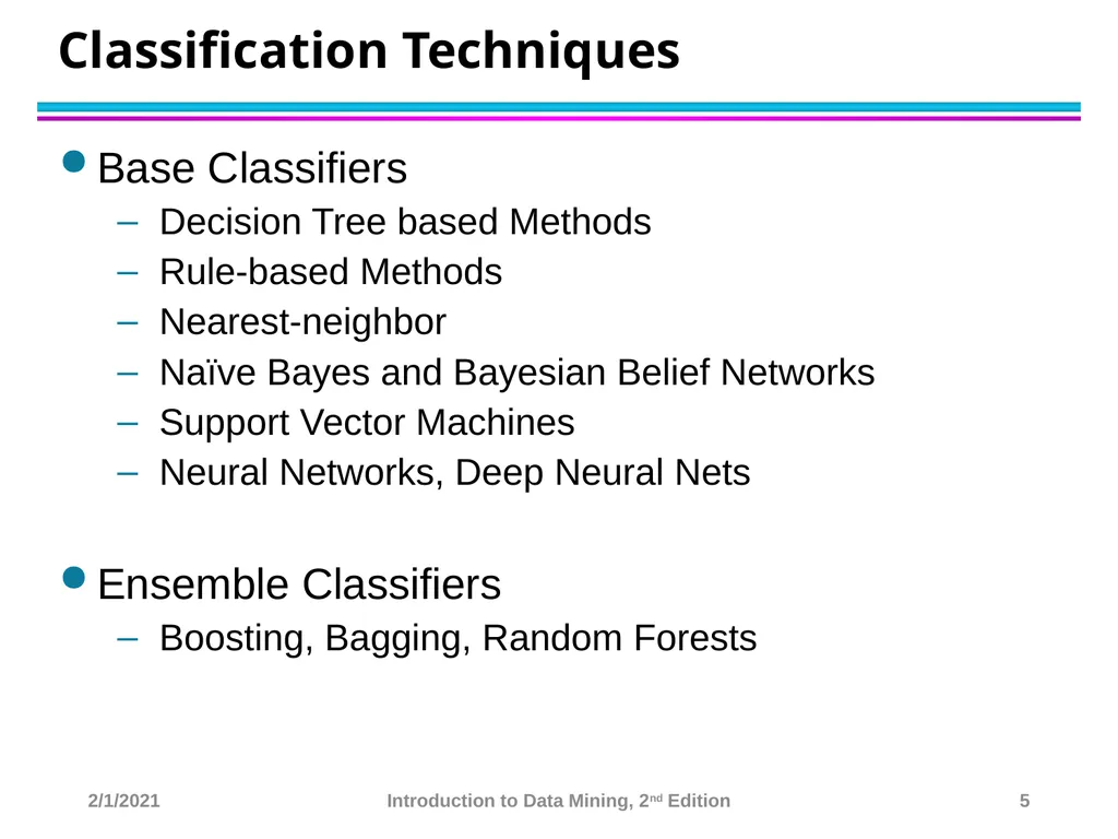
Classification Techniques Base Classifiers
Decision Tree based Methods
Rule-based Methods
Nearest-neighbor
Naïve Bayes and Bayesian Belief Networks
Support Vector Machines
Neural Networks, Deep Neural Nets
Ensemble Classifiers
Boosting, Bagging, Random Forests 2/1/2021 Introduction to Data Mining, 2nd Edition 5<br>
Decision Tree based Methods
Rule-based Methods
Nearest-neighbor
Naïve Bayes and Bayesian Belief Networks
Support Vector Machines
Neural Networks, Deep Neural Nets
Ensemble Classifiers
Boosting, Bagging, Random Forests 2/1/2021 Introduction to Data Mining, 2nd Edition 5<br>
06
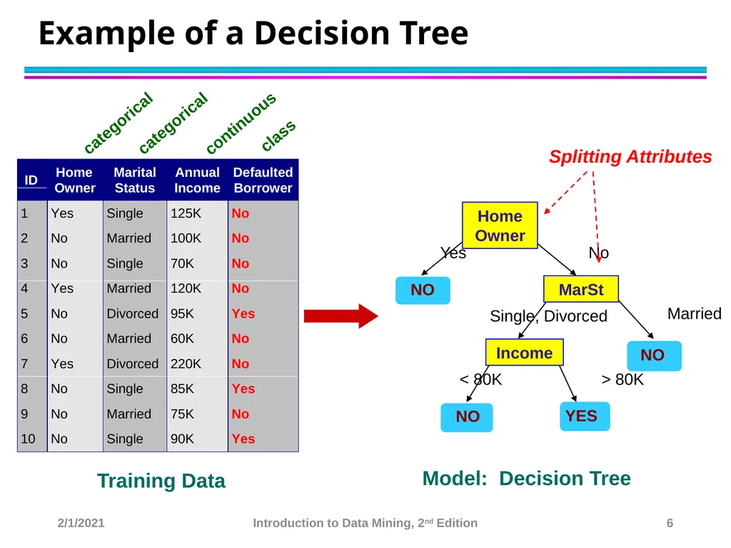
Example of a Decision Tree categorical categorical continuous class Home Owner MarSt Income YES NO NO NO Yes No Married Single, Divorced < 80K > 80K Splitting Attributes Training Data Model: Decision Tree 2/1/2021 Introduction to Data Mining, 2nd Edition 6<br>
07
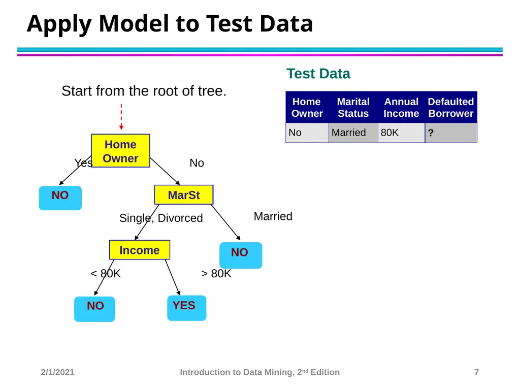
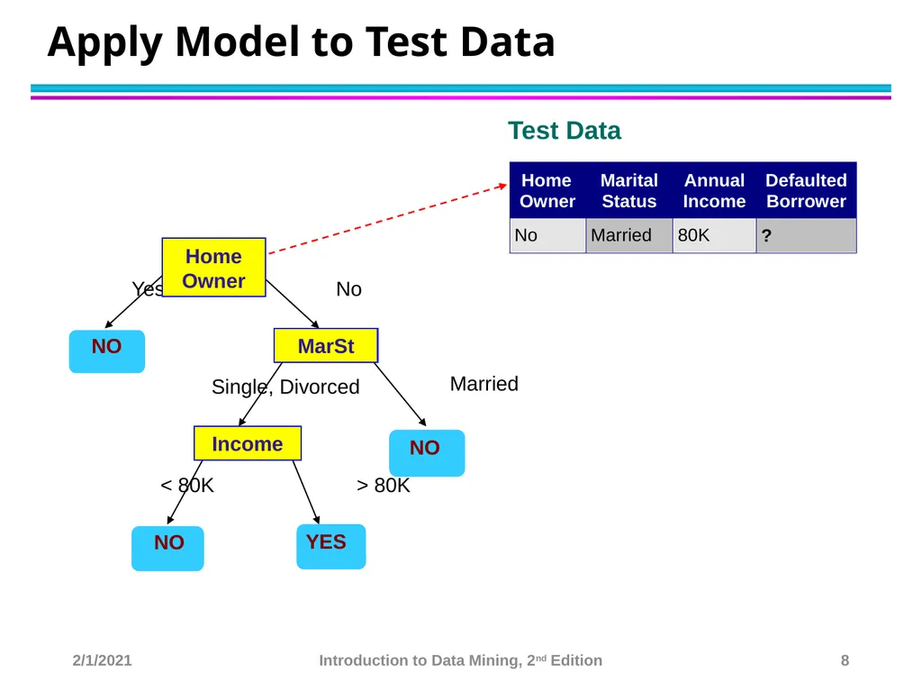
Apply Model to Test Data Home Owner MarSt Income YES NO NO NO Yes No Married Single, Divorced < 80K > 80K Test Data Start from the root of tree. 2/1/2021 Introduction to Data Mining, 2nd Edition 7<br>
08
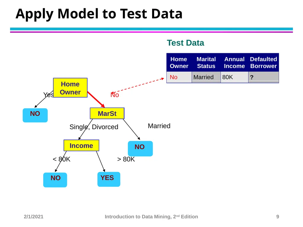
Apply Model to Test Data MarSt Income YES NO NO NO Yes No Married Single, Divorced < 80K > 80K Test Data Home Owner 2/1/2021 Introduction to Data Mining, 2nd Edition 8<br>
09
Apply Model to Test Data MarSt Income YES NO NO NO Yes No Married Single, Divorced < 80K > 80K Test Data Home Owner 2/1/2021 Introduction to Data Mining, 2nd Edition 9<br>
10
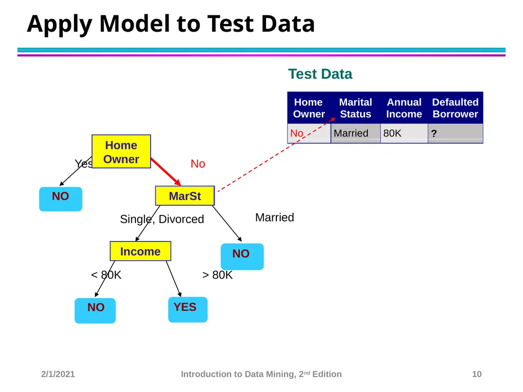
Apply Model to Test Data MarSt Income YES NO NO NO Yes No Married Single, Divorced < 80K > 80K Test Data Home Owner 2/1/2021 Introduction to Data Mining, 2nd Edition 10<br>
11
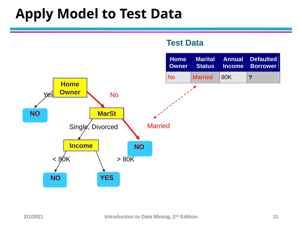
Apply Model to Test Data MarSt Income YES NO NO NO Yes No Married Single, Divorced < 80K > 80K Test Data Home Owner 2/1/2021 Introduction to Data Mining, 2nd Edition 11<br>
12
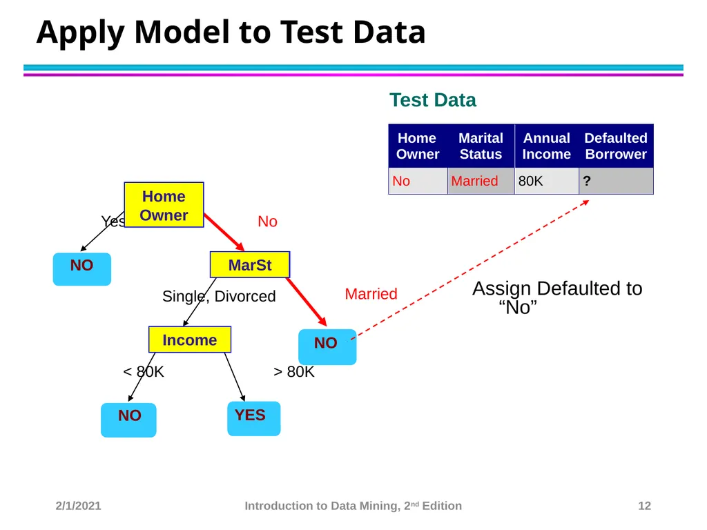
Apply Model to Test Data MarSt Income YES NO NO NO Yes No Married Single, Divorced < 80K > 80K Test Data Assign Defaulted to “No” Home Owner 2/1/2021 Introduction to Data Mining, 2nd Edition 12<br>
13
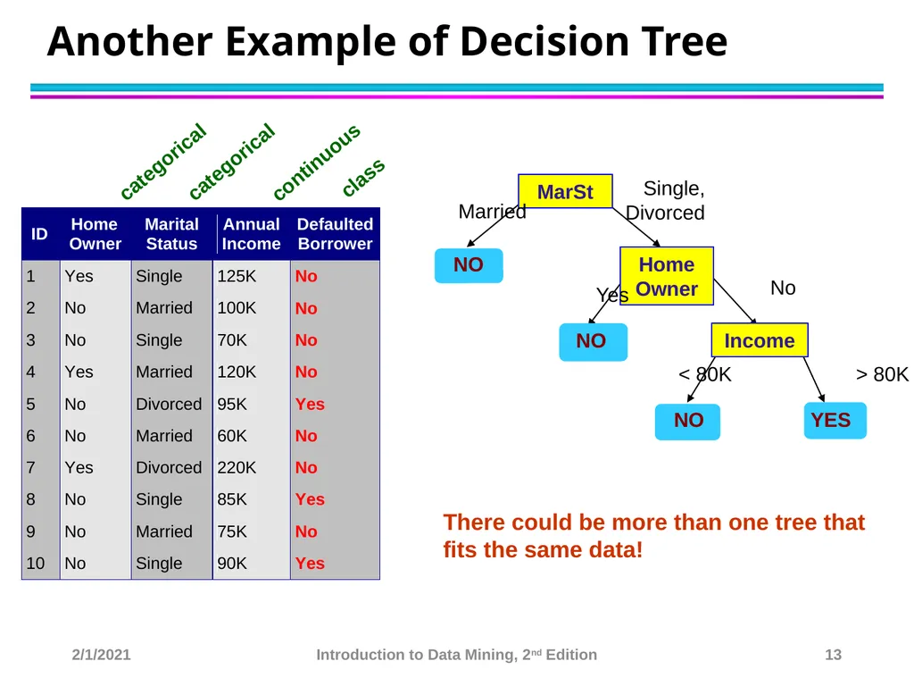
Another Example of Decision Tree categorical categorical continuous class MarSt Home Owner Income YES NO NO Yes No Married Single, Divorced < 80K > 80K There could be more than one tree that fits the same data! 2/1/2021 Introduction to Data Mining, 2nd Edition 13<br>
14
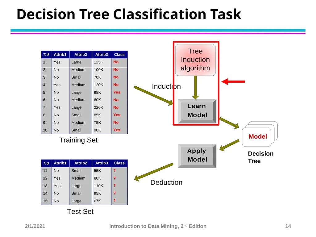
Decision Tree Classification Task Decision Tree 2/1/2021 Introduction to Data Mining, 2nd Edition 14<br>
15
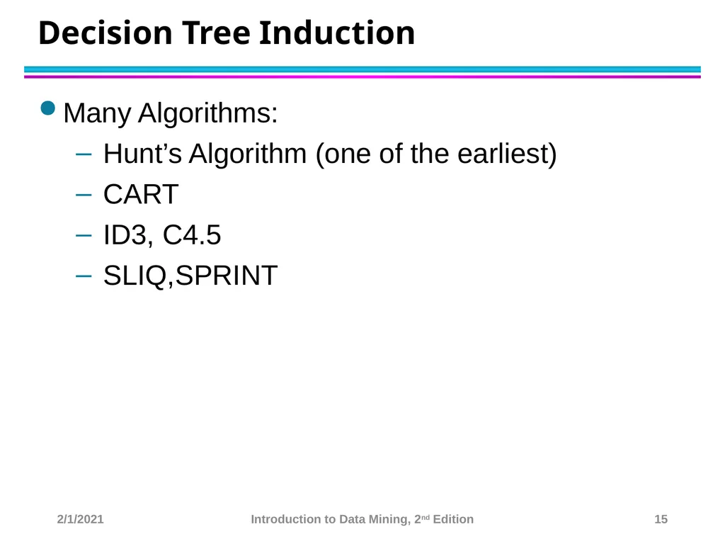
Decision Tree Induction Many Algorithms:
Hunt’s Algorithm (one of the earliest)
CART
ID3, C4.5
SLIQ,SPRINT 2/1/2021 Introduction to Data Mining, 2nd Edition 15<br>
Hunt’s Algorithm (one of the earliest)
CART
ID3, C4.5
SLIQ,SPRINT 2/1/2021 Introduction to Data Mining, 2nd Edition 15<br>
16
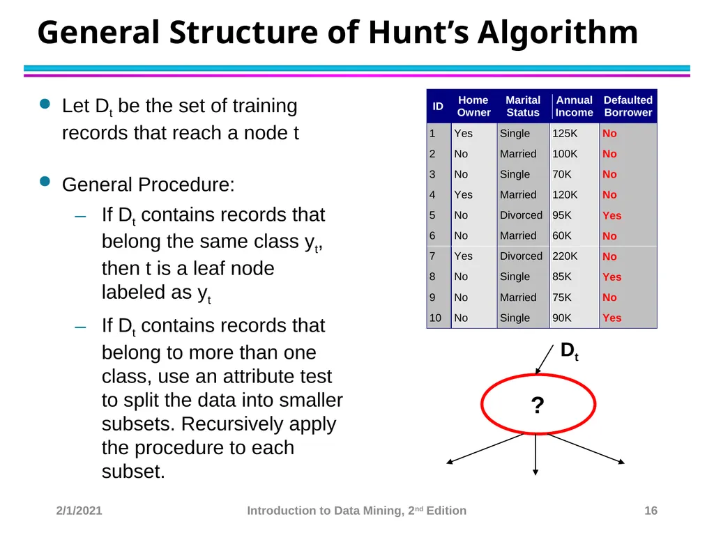
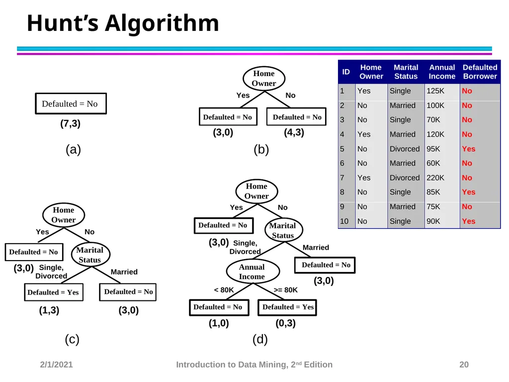
General Structure of Hunt’s Algorithm Let Dt be the set of training records that reach a node t
General Procedure:
If Dt contains records that belong the same class yt, then t is a leaf node labeled as yt
If Dt contains records that belong to more than one class, use an attribute test to split the data into smaller subsets. Recursively apply the procedure to each subset. Dt ? 2/1/2021 Introduction to Data Mining, 2nd Edition 16<br>
General Procedure:
If Dt contains records that belong the same class yt, then t is a leaf node labeled as yt
If Dt contains records that belong to more than one class, use an attribute test to split the data into smaller subsets. Recursively apply the procedure to each subset. Dt ? 2/1/2021 Introduction to Data Mining, 2nd Edition 16<br>
17
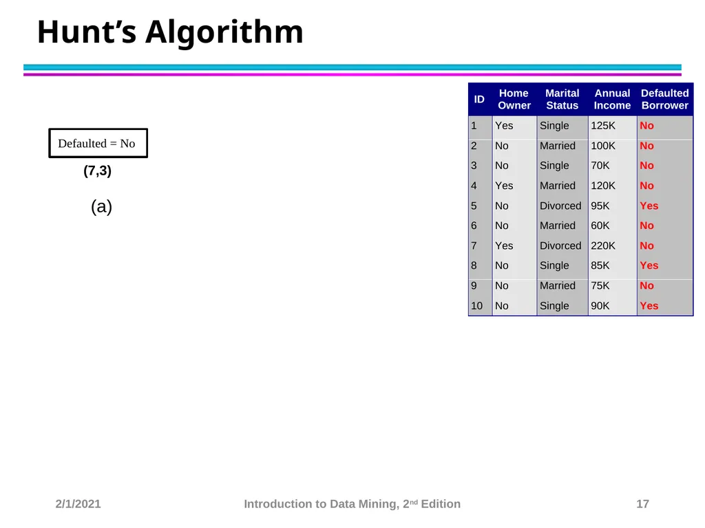
Hunt’s Algorithm (3,0) (4,3) (3,0) (1,3) (3,0) (3,0) (1,0) (0,3) (3,0) (7,3) 2/1/2021 Introduction to Data Mining, 2nd Edition 17<br>
18
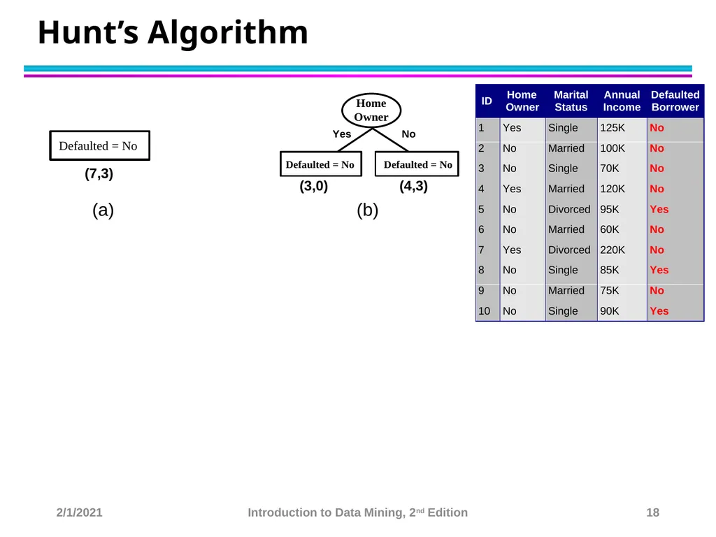
Hunt’s Algorithm (3,0) (4,3) (3,0) (1,3) (3,0) (3,0) (1,0) (0,3) (3,0) (7,3) 2/1/2021 Introduction to Data Mining, 2nd Edition 18<br>
19
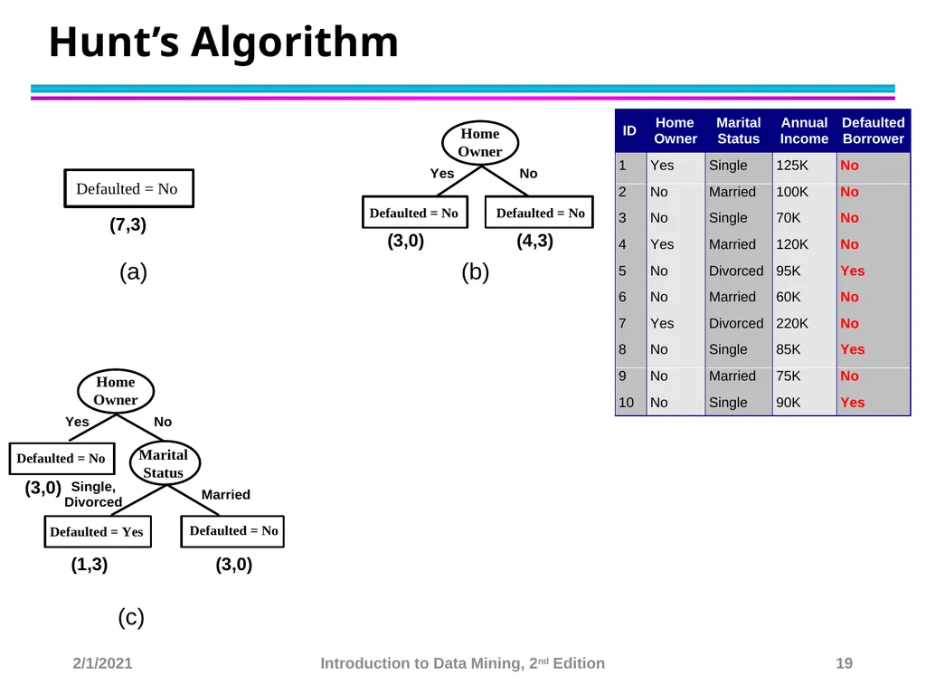
Hunt’s Algorithm (3,0) (4,3) (3,0) (1,3) (3,0) (3,0) (1,0) (0,3) (3,0) (7,3) 2/1/2021 Introduction to Data Mining, 2nd Edition 19<br>
20
Hunt’s Algorithm (3,0) (4,3) (3,0) (1,3) (3,0) (3,0) (1,0) (0,3) (3,0) (7,3) 2/1/2021 Introduction to Data Mining, 2nd Edition 20<br>
21
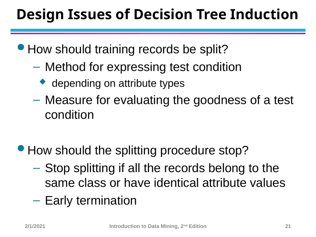
Design Issues of Decision Tree Induction How should training records be split?
Method for expressing test condition
depending on attribute types
Measure for evaluating the goodness of a test condition
How should the splitting procedure stop?
Stop splitting if all the records belong to the same class or have identical attribute values
Early termination 2/1/2021 Introduction to Data Mining, 2nd Edition 21<br>
Method for expressing test condition
depending on attribute types
Measure for evaluating the goodness of a test condition
How should the splitting procedure stop?
Stop splitting if all the records belong to the same class or have identical attribute values
Early termination 2/1/2021 Introduction to Data Mining, 2nd Edition 21<br>
22
Methods for Expressing Test Conditions Depends on attribute types
Binary
Nominal
Ordinal
Continuous 2/1/2021 Introduction to Data Mining, 2nd Edition 22<br>
Binary
Nominal
Ordinal
Continuous 2/1/2021 Introduction to Data Mining, 2nd Edition 22<br>
23
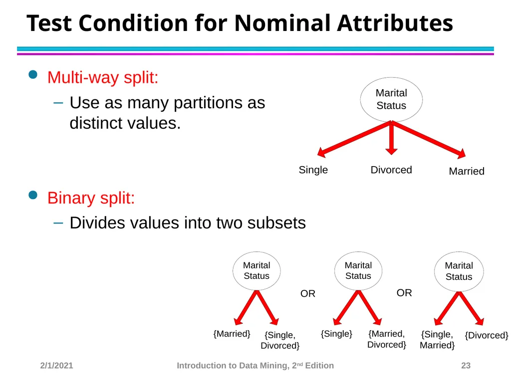
Test Condition for Nominal Attributes Multi-way split:
Use as many partitions as distinct values.
Binary split:
Divides values into two subsets 2/1/2021 Introduction to Data Mining, 2nd Edition 23<br>
Use as many partitions as distinct values.
Binary split:
Divides values into two subsets 2/1/2021 Introduction to Data Mining, 2nd Edition 23<br>
24
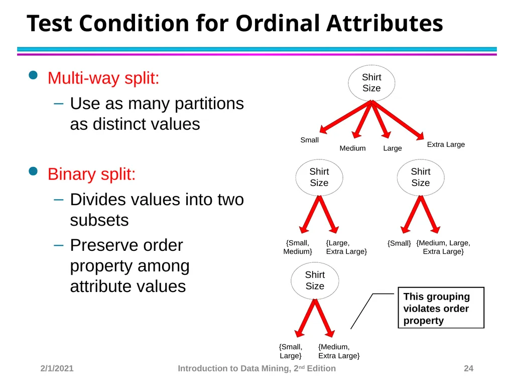
Test Condition for Ordinal Attributes Multi-way split:
Use as many partitions as distinct values
Binary split:
Divides values into two subsets
Preserve order property among attribute values This grouping violates order property 2/1/2021 Introduction to Data Mining, 2nd Edition 24<br>
Use as many partitions as distinct values
Binary split:
Divides values into two subsets
Preserve order property among attribute values This grouping violates order property 2/1/2021 Introduction to Data Mining, 2nd Edition 24<br>
25
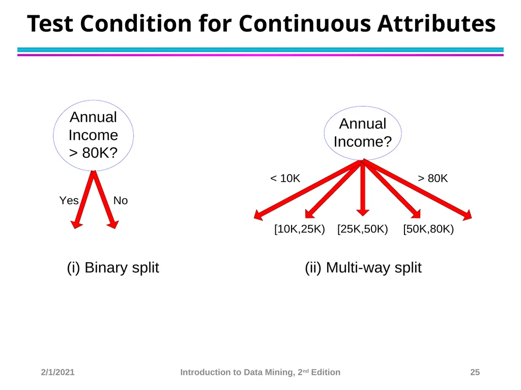
Test Condition for Continuous Attributes 2/1/2021 Introduction to Data Mining, 2nd Edition 25<br>
26
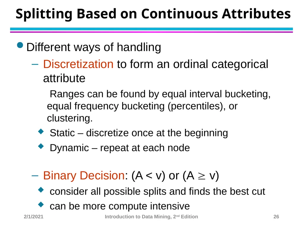
Splitting Based on Continuous Attributes Different ways of handling
Discretization to form an ordinal categorical attribute
Ranges can be found by equal interval bucketing, equal frequency bucketing (percentiles), or clustering.
Static – discretize once at the beginning
Dynamic – repeat at each node
Binary Decision: (A < v) or (A v)
consider all possible splits and finds the best cut
can be more compute intensive 2/1/2021 Introduction to Data Mining, 2nd Edition 26<br>
Discretization to form an ordinal categorical attribute
Ranges can be found by equal interval bucketing, equal frequency bucketing (percentiles), or clustering.
Static – discretize once at the beginning
Dynamic – repeat at each node
Binary Decision: (A < v) or (A v)
consider all possible splits and finds the best cut
can be more compute intensive 2/1/2021 Introduction to Data Mining, 2nd Edition 26<br>
27
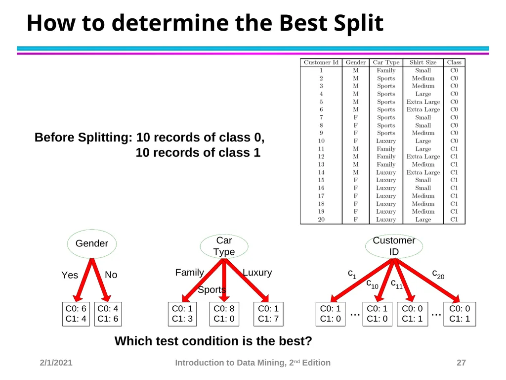
How to determine the Best Split Before Splitting: 10 records of class 0,
10 records of class 1 Which test condition is the best? 2/1/2021 Introduction to Data Mining, 2nd Edition 27<br>
28
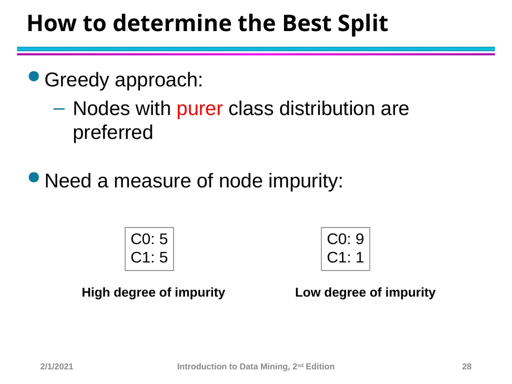
How to determine the Best Split Greedy approach:
Nodes with purer class distribution are preferred
Need a measure of node impurity: High degree of impurity Low degree of impurity 2/1/2021 Introduction to Data Mining, 2nd Edition 28<br>
Nodes with purer class distribution are preferred
Need a measure of node impurity: High degree of impurity Low degree of impurity 2/1/2021 Introduction to Data Mining, 2nd Edition 28<br>
29
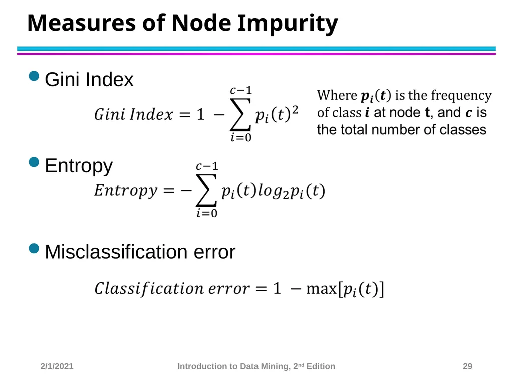
Measures of Node Impurity Gini Index
Entropy
Misclassification error 2/1/2021 Introduction to Data Mining, 2nd Edition 29<br>
Entropy
Misclassification error 2/1/2021 Introduction to Data Mining, 2nd Edition 29<br>
30
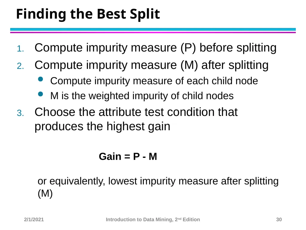
Finding the Best Split Compute impurity measure (P) before splitting
Compute impurity measure (M) after splitting
Compute impurity measure of each child node
M is the weighted impurity of child nodes
Choose the attribute test condition that produces the highest gain
Gain = P - M or equivalently, lowest impurity measure after splitting (M) 2/1/2021 Introduction to Data Mining, 2nd Edition 30<br>
Compute impurity measure (M) after splitting
Compute impurity measure of each child node
M is the weighted impurity of child nodes
Choose the attribute test condition that produces the highest gain
Gain = P - M or equivalently, lowest impurity measure after splitting (M) 2/1/2021 Introduction to Data Mining, 2nd Edition 30<br>
31
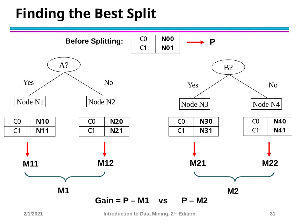
Finding the Best Split B? Yes No Node N3 Node N4 A? Yes No Node N1 Node N2 Before Splitting: Gain = P – M1 vs P – M2 2/1/2021 Introduction to Data Mining, 2nd Edition 31<br>
32
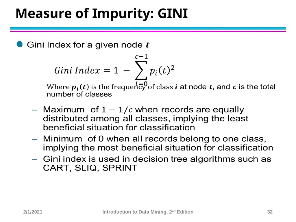
Measure of Impurity: GINI 2/1/2021 Introduction to Data Mining, 2nd Edition 32<br>
33
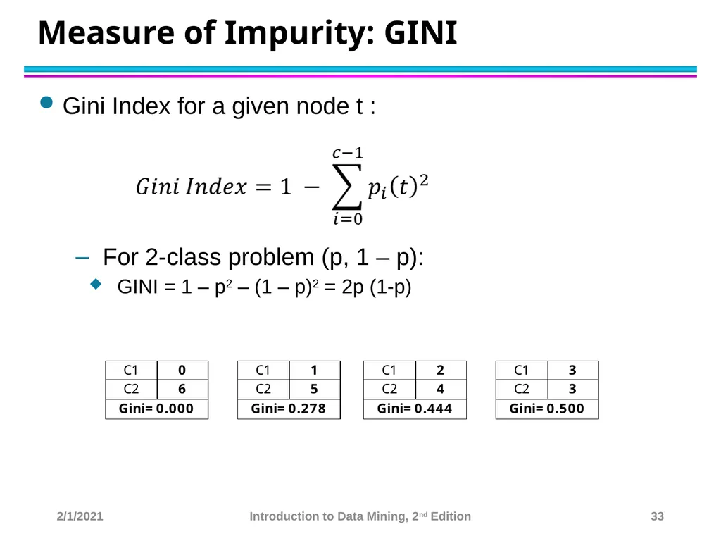
Measure of Impurity: GINI Gini Index for a given node t :
For 2-class problem (p, 1 – p):
GINI = 1 – p2 – (1 – p)2 = 2p (1-p) 2/1/2021 Introduction to Data Mining, 2nd Edition 33<br>
For 2-class problem (p, 1 – p):
GINI = 1 – p2 – (1 – p)2 = 2p (1-p) 2/1/2021 Introduction to Data Mining, 2nd Edition 33<br>
34
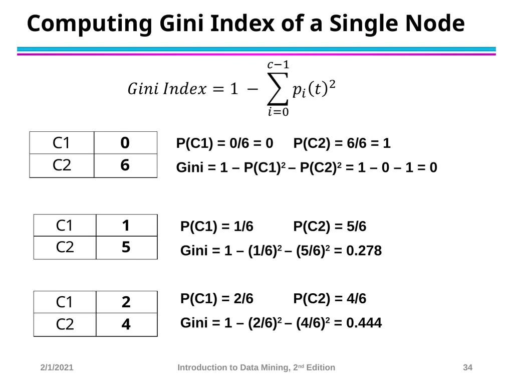
Computing Gini Index of a Single Node P(C1) = 0/6 = 0 P(C2) = 6/6 = 1
Gini = 1 – P(C1)2 – P(C2)2 = 1 – 0 – 1 = 0 P(C1) = 1/6 P(C2) = 5/6
Gini = 1 – (1/6)2 – (5/6)2 = 0.278 P(C1) = 2/6 P(C2) = 4/6
Gini = 1 – (2/6)2 – (4/6)2 = 0.444 2/1/2021 Introduction to Data Mining, 2nd Edition 34<br>
Gini = 1 – P(C1)2 – P(C2)2 = 1 – 0 – 1 = 0 P(C1) = 1/6 P(C2) = 5/6
Gini = 1 – (1/6)2 – (5/6)2 = 0.278 P(C1) = 2/6 P(C2) = 4/6
Gini = 1 – (2/6)2 – (4/6)2 = 0.444 2/1/2021 Introduction to Data Mining, 2nd Edition 34<br>
35
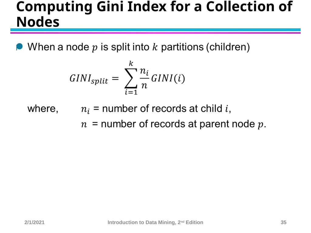
Computing Gini Index for a Collection of Nodes 2/1/2021 Introduction to Data Mining, 2nd Edition 35<br>
36
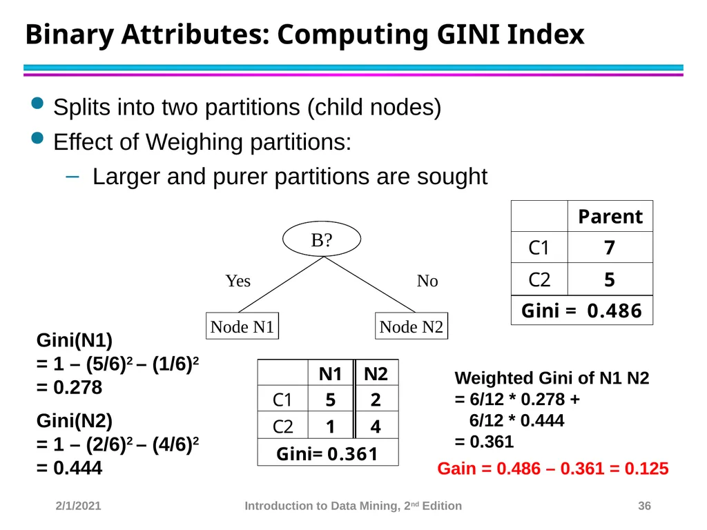
Binary Attributes: Computing GINI Index Splits into two partitions (child nodes)
Effect of Weighing partitions:
Larger and purer partitions are sought B? Yes No Node N1 Node N2 Gini(N1) = 1 – (5/6)2 – (1/6)2 = 0.278
Gini(N2) = 1 – (2/6)2 – (4/6)2 = 0.444 Weighted Gini of N1 N2 = 6/12 * 0.278 + 6/12 * 0.444 = 0.361 Gain = 0.486 – 0.361 = 0.125 2/1/2021 Introduction to Data Mining, 2nd Edition 36<br>
Effect of Weighing partitions:
Larger and purer partitions are sought B? Yes No Node N1 Node N2 Gini(N1) = 1 – (5/6)2 – (1/6)2 = 0.278
Gini(N2) = 1 – (2/6)2 – (4/6)2 = 0.444 Weighted Gini of N1 N2 = 6/12 * 0.278 + 6/12 * 0.444 = 0.361 Gain = 0.486 – 0.361 = 0.125 2/1/2021 Introduction to Data Mining, 2nd Edition 36<br>
37
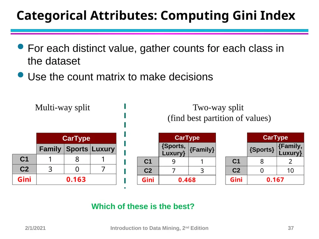
Categorical Attributes: Computing Gini Index For each distinct value, gather counts for each class in the dataset
Use the count matrix to make decisions Multi-way split Two-way split
(find best partition of values) Which of these is the best? 2/1/2021 Introduction to Data Mining, 2nd Edition 37<br>
Use the count matrix to make decisions Multi-way split Two-way split
(find best partition of values) Which of these is the best? 2/1/2021 Introduction to Data Mining, 2nd Edition 37<br>
38
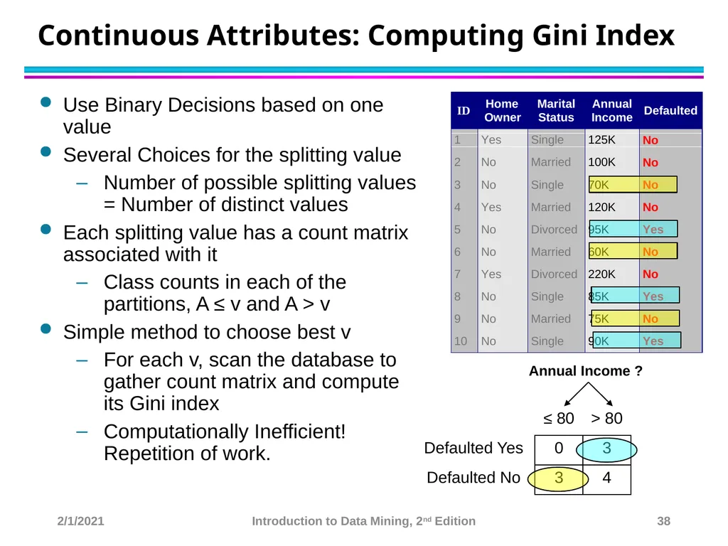
Continuous Attributes: Computing Gini Index Use Binary Decisions based on one value
Several Choices for the splitting value
Number of possible splitting values = Number of distinct values
Each splitting value has a count matrix associated with it
Class counts in each of the partitions, A ≤ v and A > v
Simple method to choose best v
For each v, scan the database to gather count matrix and compute its Gini index
Computationally Inefficient! Repetition of work. Annual Income ? 2/1/2021 Introduction to Data Mining, 2nd Edition 38<br>
Several Choices for the splitting value
Number of possible splitting values = Number of distinct values
Each splitting value has a count matrix associated with it
Class counts in each of the partitions, A ≤ v and A > v
Simple method to choose best v
For each v, scan the database to gather count matrix and compute its Gini index
Computationally Inefficient! Repetition of work. Annual Income ? 2/1/2021 Introduction to Data Mining, 2nd Edition 38<br>
39
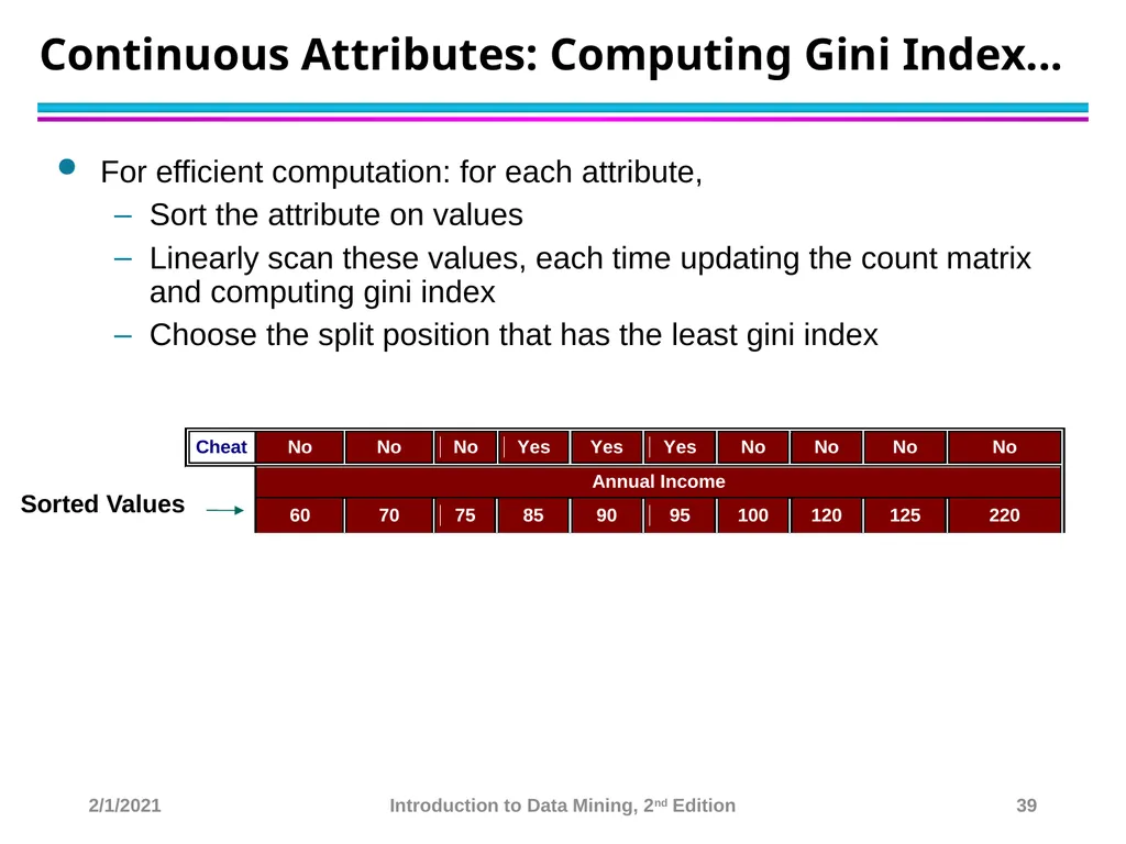
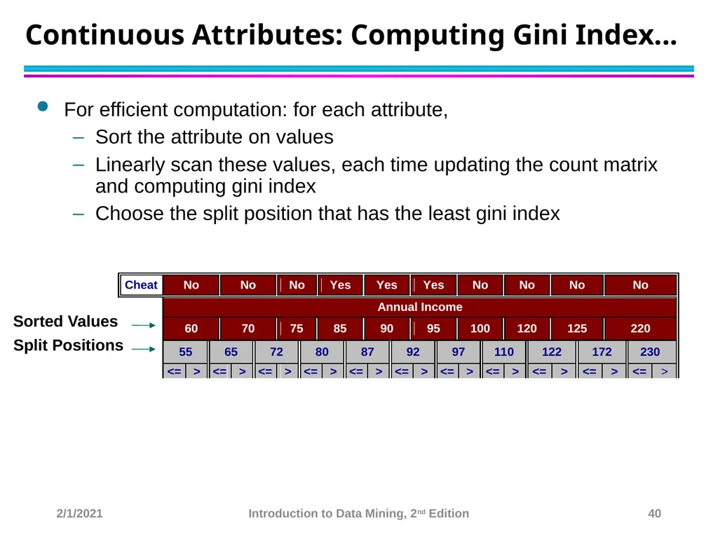
Continuous Attributes: Computing Gini Index... For efficient computation: for each attribute,
Sort the attribute on values
Linearly scan these values, each time updating the count matrix and computing gini index
Choose the split position that has the least gini index Sorted Values 2/1/2021 Introduction to Data Mining, 2nd Edition 39<br>
Sort the attribute on values
Linearly scan these values, each time updating the count matrix and computing gini index
Choose the split position that has the least gini index Sorted Values 2/1/2021 Introduction to Data Mining, 2nd Edition 39<br>
40
Continuous Attributes: Computing Gini Index... For efficient computation: for each attribute,
Sort the attribute on values
Linearly scan these values, each time updating the count matrix and computing gini index
Choose the split position that has the least gini index Sorted Values 2/1/2021 Introduction to Data Mining, 2nd Edition 40<br>
Sort the attribute on values
Linearly scan these values, each time updating the count matrix and computing gini index
Choose the split position that has the least gini index Sorted Values 2/1/2021 Introduction to Data Mining, 2nd Edition 40<br>
41
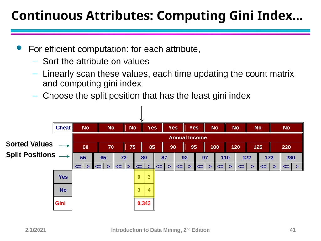
Continuous Attributes: Computing Gini Index... For efficient computation: for each attribute,
Sort the attribute on values
Linearly scan these values, each time updating the count matrix and computing gini index
Choose the split position that has the least gini index Sorted Values 2/1/2021 Introduction to Data Mining, 2nd Edition 41<br>
Sort the attribute on values
Linearly scan these values, each time updating the count matrix and computing gini index
Choose the split position that has the least gini index Sorted Values 2/1/2021 Introduction to Data Mining, 2nd Edition 41<br>
42
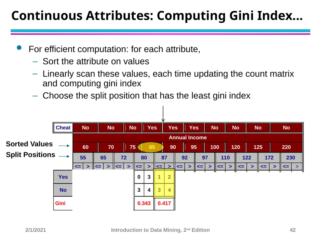
Continuous Attributes: Computing Gini Index... For efficient computation: for each attribute,
Sort the attribute on values
Linearly scan these values, each time updating the count matrix and computing gini index
Choose the split position that has the least gini index Sorted Values 2/1/2021 Introduction to Data Mining, 2nd Edition 42<br>
Sort the attribute on values
Linearly scan these values, each time updating the count matrix and computing gini index
Choose the split position that has the least gini index Sorted Values 2/1/2021 Introduction to Data Mining, 2nd Edition 42<br>
43
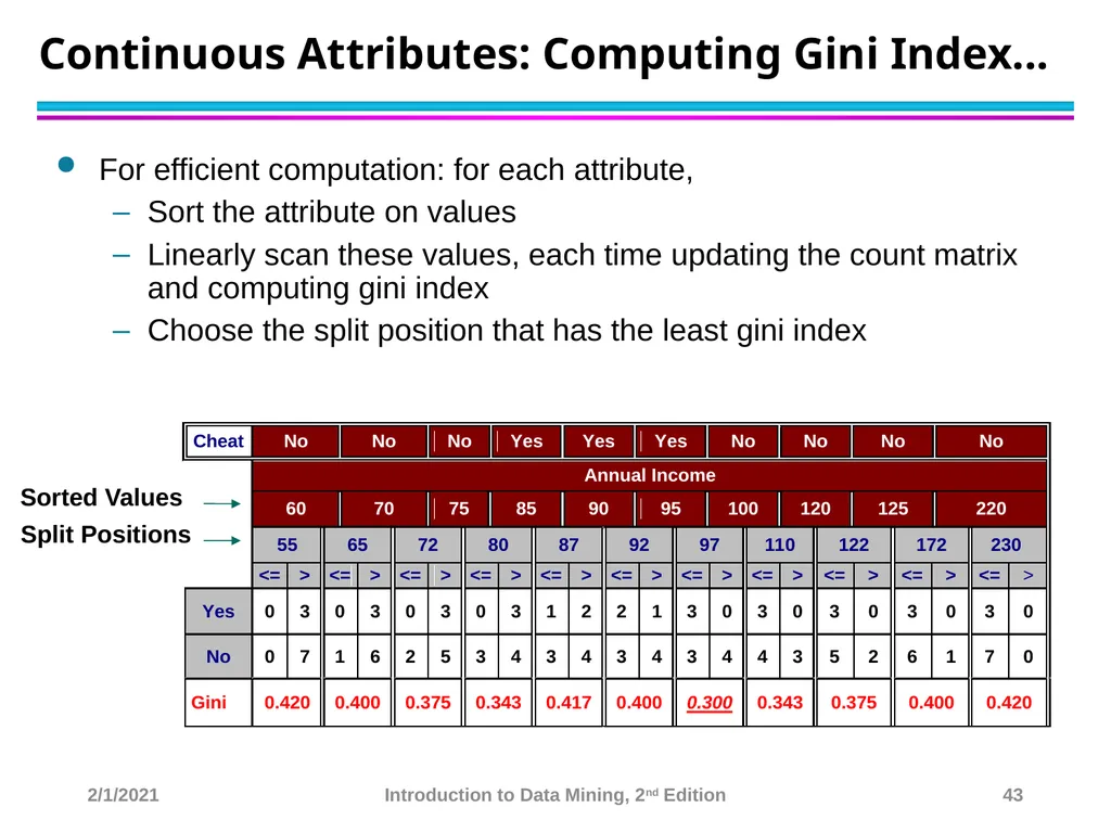
Continuous Attributes: Computing Gini Index... For efficient computation: for each attribute,
Sort the attribute on values
Linearly scan these values, each time updating the count matrix and computing gini index
Choose the split position that has the least gini index Sorted Values 2/1/2021 Introduction to Data Mining, 2nd Edition 43<br>
Sort the attribute on values
Linearly scan these values, each time updating the count matrix and computing gini index
Choose the split position that has the least gini index Sorted Values 2/1/2021 Introduction to Data Mining, 2nd Edition 43<br>
44
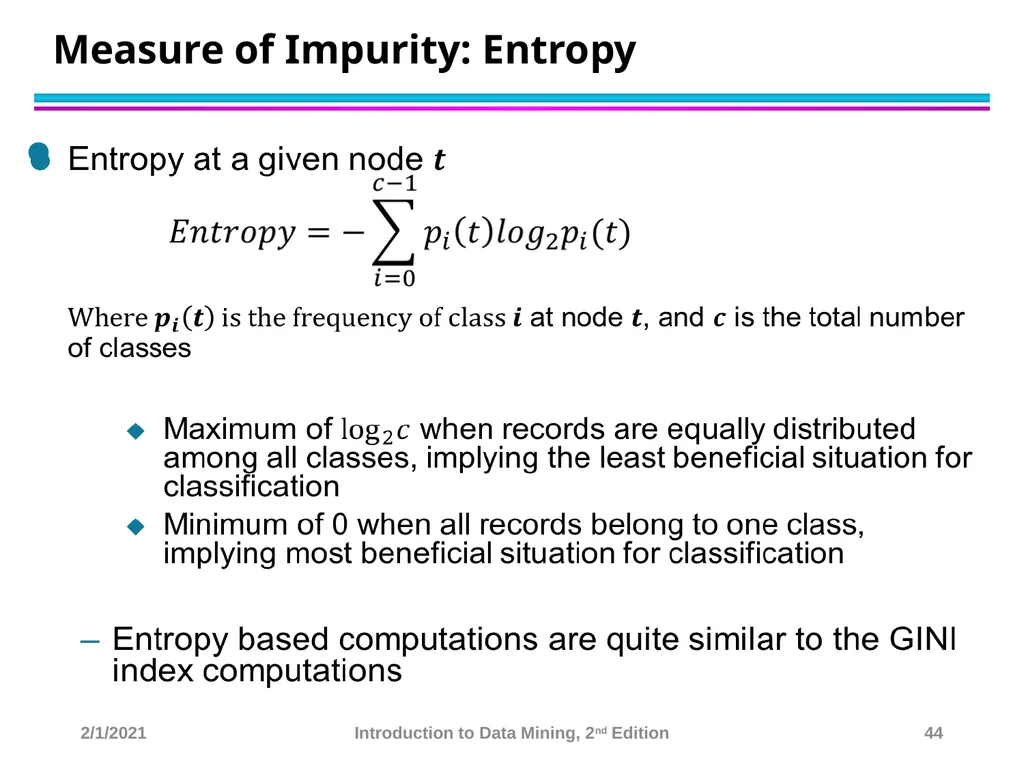
Measure of Impurity: Entropy 2/1/2021 Introduction to Data Mining, 2nd Edition 44<br>
45
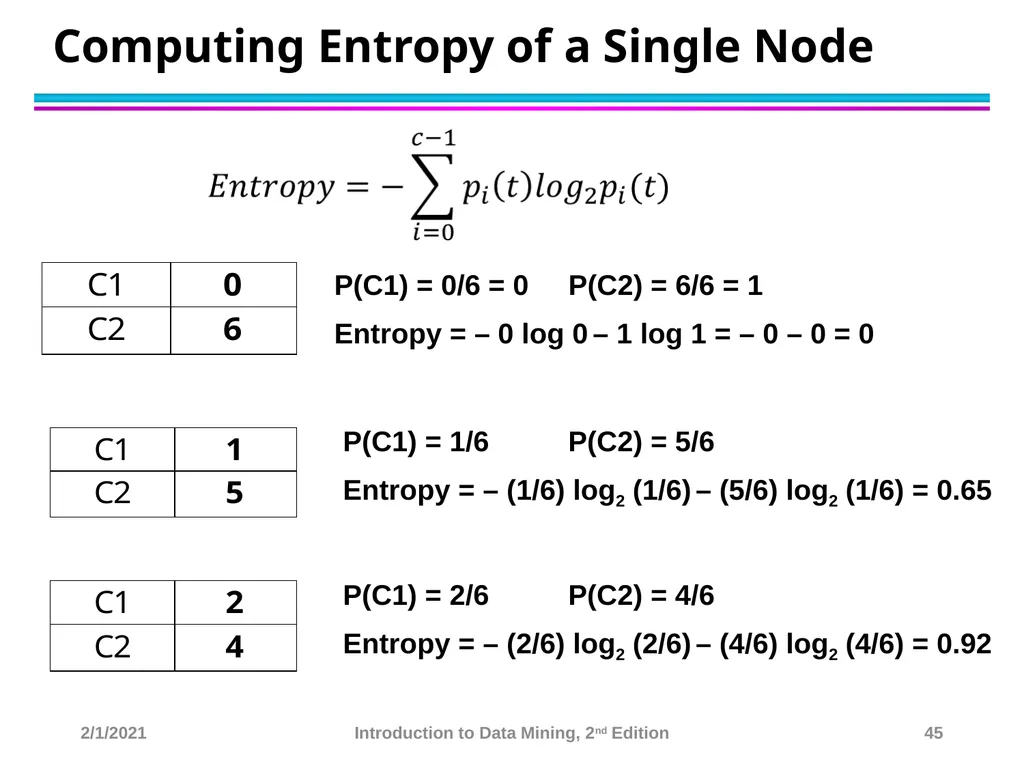
Computing Entropy of a Single Node P(C1) = 0/6 = 0 P(C2) = 6/6 = 1
Entropy = – 0 log 0 – 1 log 1 = – 0 – 0 = 0 P(C1) = 1/6 P(C2) = 5/6
Entropy = – (1/6) log2 (1/6) – (5/6) log2 (1/6) = 0.65 P(C1) = 2/6 P(C2) = 4/6
Entropy = – (2/6) log2 (2/6) – (4/6) log2 (4/6) = 0.92 2/1/2021 Introduction to Data Mining, 2nd Edition 45<br>
Entropy = – 0 log 0 – 1 log 1 = – 0 – 0 = 0 P(C1) = 1/6 P(C2) = 5/6
Entropy = – (1/6) log2 (1/6) – (5/6) log2 (1/6) = 0.65 P(C1) = 2/6 P(C2) = 4/6
Entropy = – (2/6) log2 (2/6) – (4/6) log2 (4/6) = 0.92 2/1/2021 Introduction to Data Mining, 2nd Edition 45<br>
46
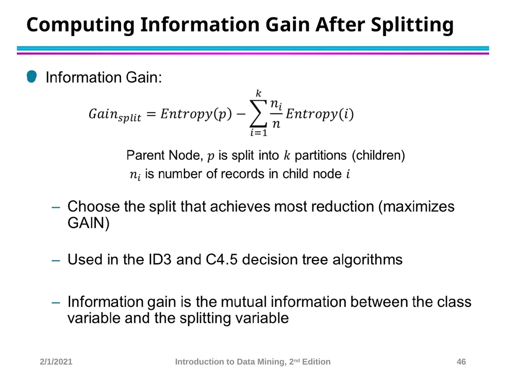
Computing Information Gain After Splitting 2/1/2021 Introduction to Data Mining, 2nd Edition 46<br>
47
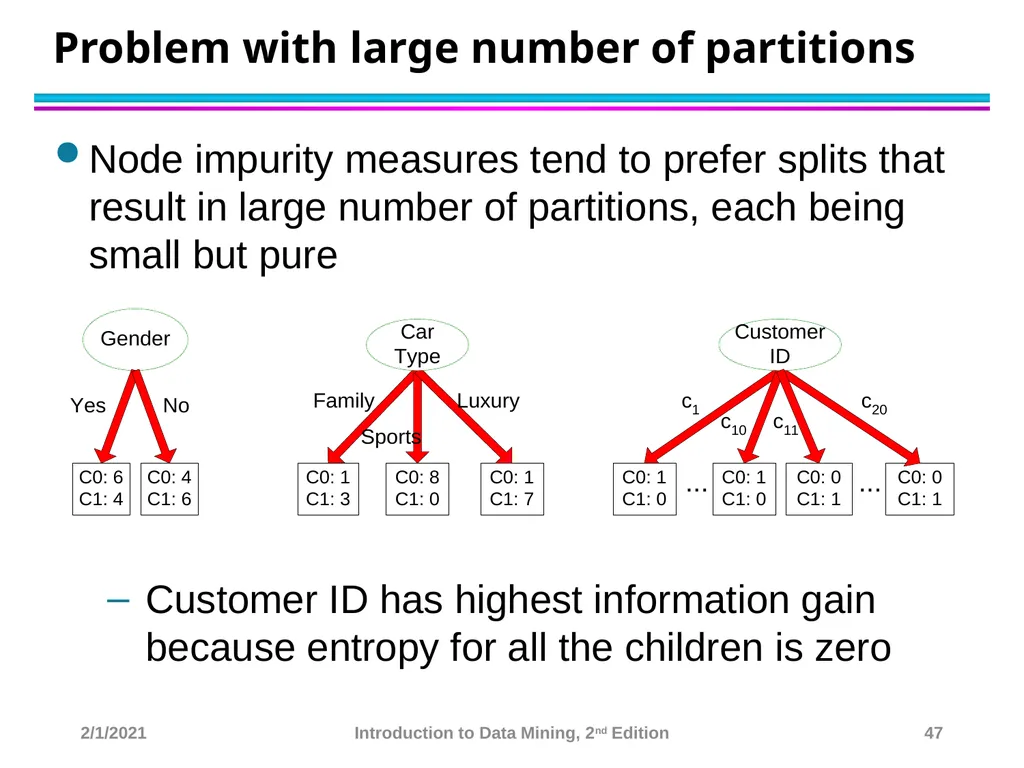
Problem with large number of partitions Node impurity measures tend to prefer splits that result in large number of partitions, each being small but pure
Customer ID has highest information gain because entropy for all the children is zero 2/1/2021 Introduction to Data Mining, 2nd Edition 47<br>
Customer ID has highest information gain because entropy for all the children is zero 2/1/2021 Introduction to Data Mining, 2nd Edition 47<br>
48
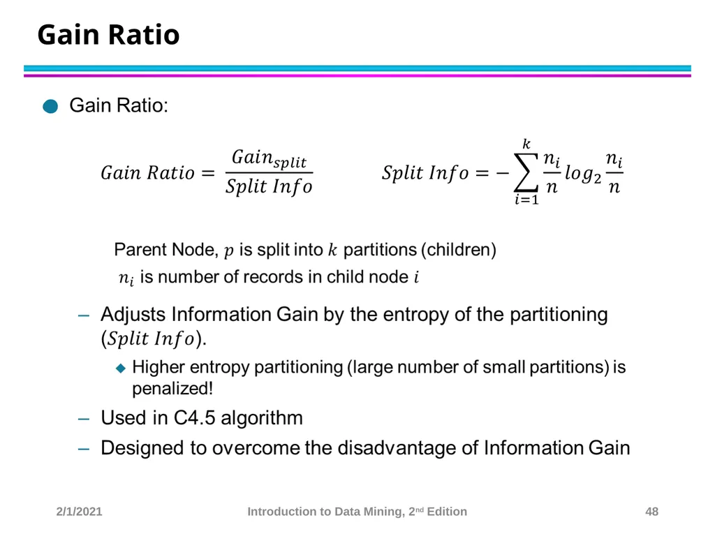
Gain Ratio 2/1/2021 Introduction to Data Mining, 2nd Edition 48<br>
49
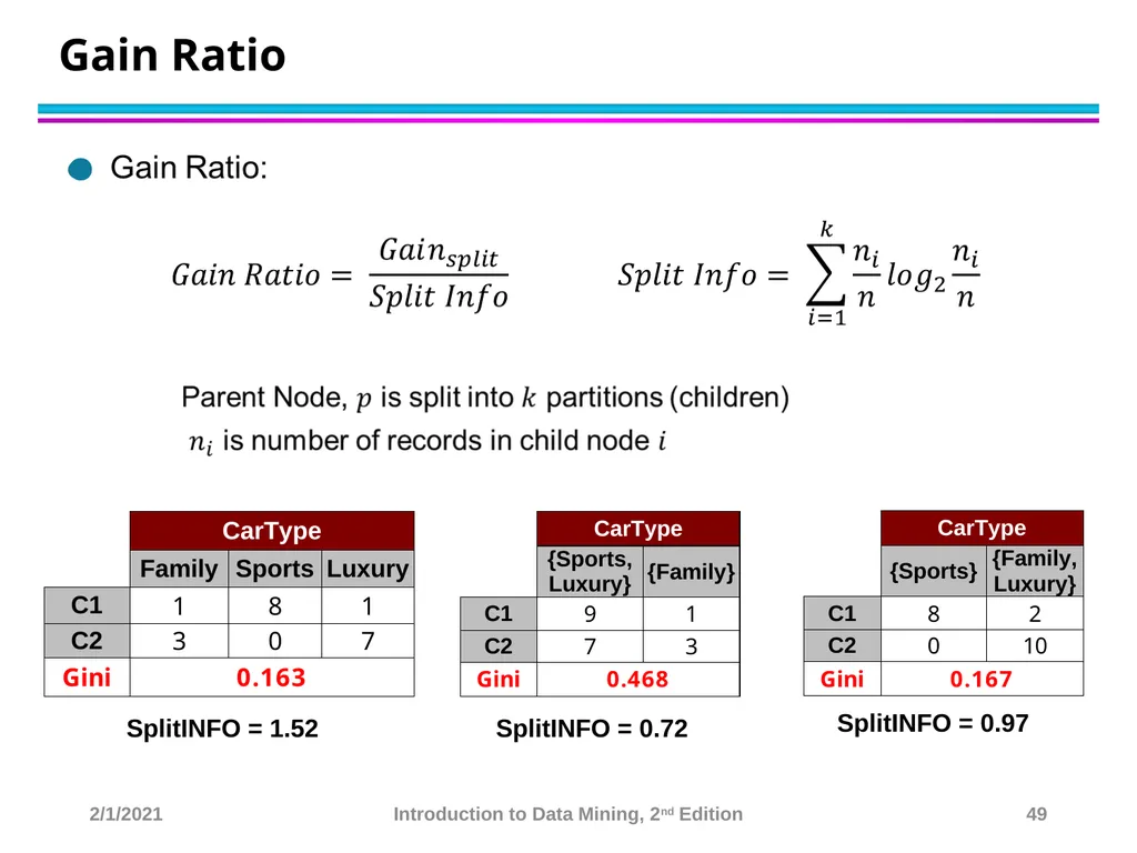
Gain Ratio SplitINFO = 1.52 SplitINFO = 0.72 SplitINFO = 0.97 2/1/2021 Introduction to Data Mining, 2nd Edition 49<br>
50
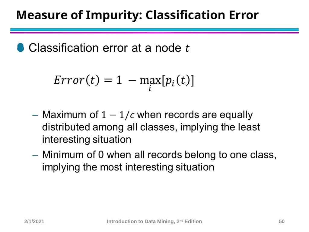
Measure of Impurity: Classification Error 2/1/2021 Introduction to Data Mining, 2nd Edition 50<br>
51
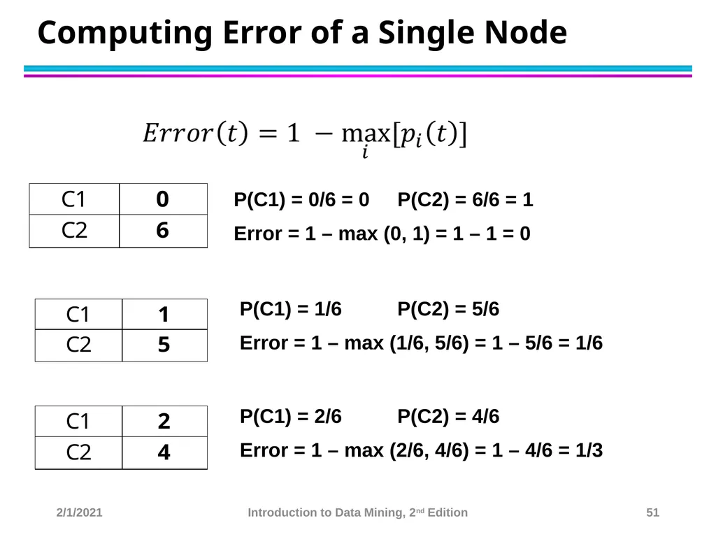
Computing Error of a Single Node P(C1) = 0/6 = 0 P(C2) = 6/6 = 1
Error = 1 – max (0, 1) = 1 – 1 = 0 P(C1) = 1/6 P(C2) = 5/6
Error = 1 – max (1/6, 5/6) = 1 – 5/6 = 1/6 P(C1) = 2/6 P(C2) = 4/6
Error = 1 – max (2/6, 4/6) = 1 – 4/6 = 1/3 2/1/2021 Introduction to Data Mining, 2nd Edition 51<br>
Error = 1 – max (0, 1) = 1 – 1 = 0 P(C1) = 1/6 P(C2) = 5/6
Error = 1 – max (1/6, 5/6) = 1 – 5/6 = 1/6 P(C1) = 2/6 P(C2) = 4/6
Error = 1 – max (2/6, 4/6) = 1 – 4/6 = 1/3 2/1/2021 Introduction to Data Mining, 2nd Edition 51<br>
52
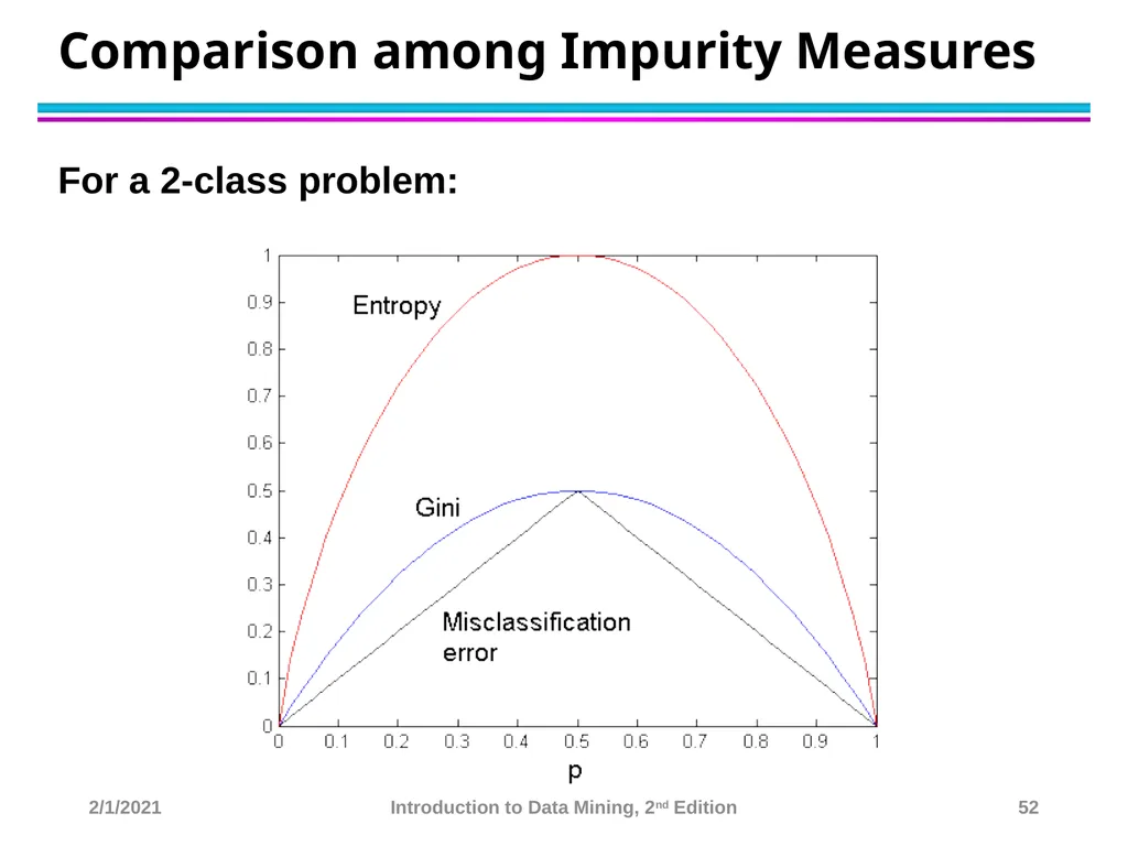
Comparison among Impurity Measures For a 2-class problem: 2/1/2021 Introduction to Data Mining, 2nd Edition 52<br>
53
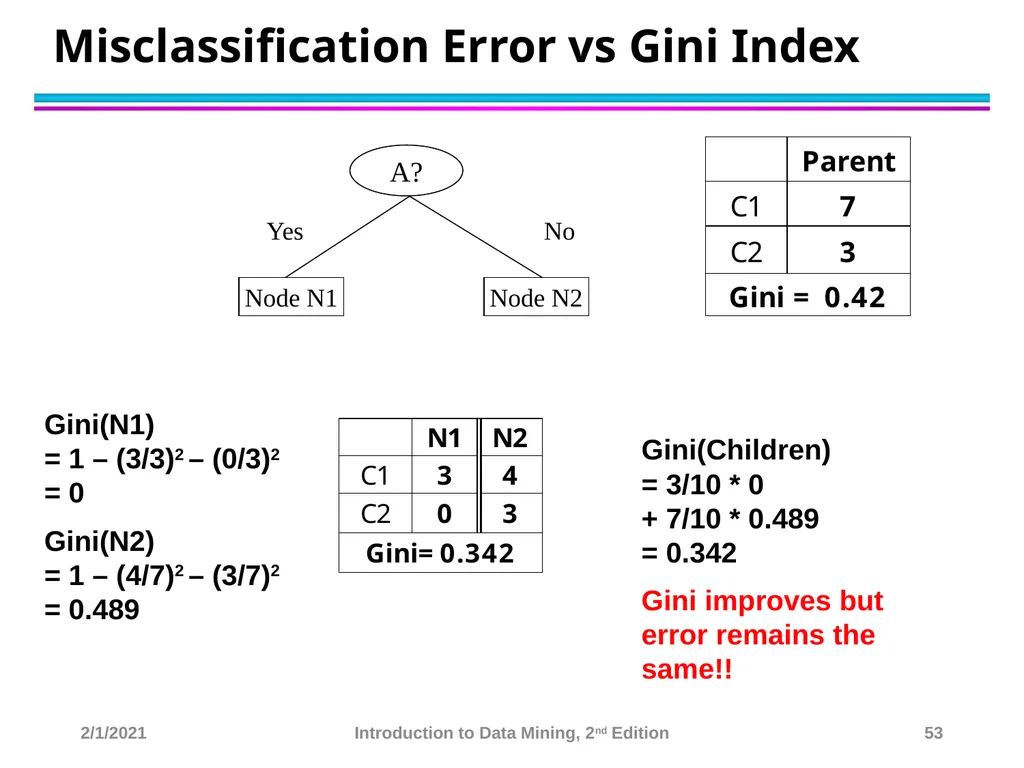
Misclassification Error vs Gini Index A? Yes No Node N1 Node N2 Gini(N1)
= 1 – (3/3)2 – (0/3)2
= 0
Gini(N2) = 1 – (4/7)2 – (3/7)2 = 0.489 Gini(Children) = 3/10 * 0 + 7/10 * 0.489 = 0.342
Gini improves but error remains the same!! 2/1/2021 Introduction to Data Mining, 2nd Edition 53<br>
Gini(N2) = 1 – (4/7)2 – (3/7)2 = 0.489 Gini(Children) = 3/10 * 0 + 7/10 * 0.489 = 0.342
Gini improves but error remains the same!! 2/1/2021 Introduction to Data Mining, 2nd Edition 53<br>
54
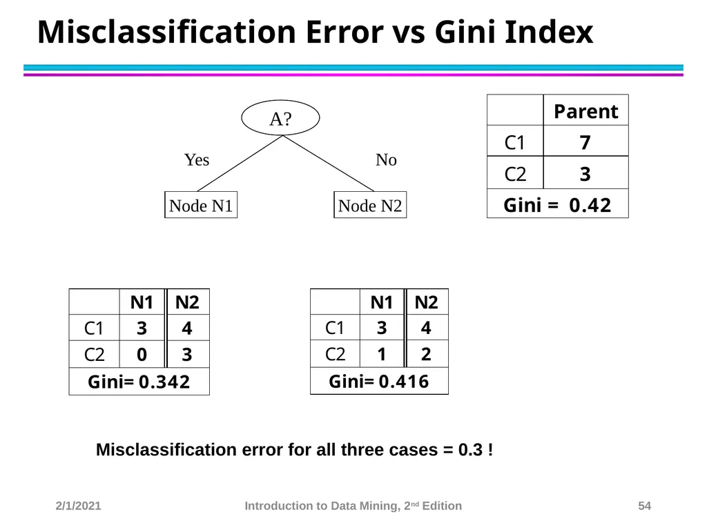
Misclassification Error vs Gini Index A? Yes No Node N1 Node N2 Misclassification error for all three cases = 0.3 ! 2/1/2021 Introduction to Data Mining, 2nd Edition 54<br>
55
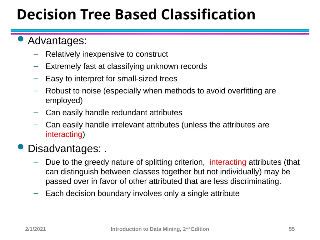
Decision Tree Based Classification Advantages:
Relatively inexpensive to construct
Extremely fast at classifying unknown records
Easy to interpret for small-sized trees
Robust to noise (especially when methods to avoid overfitting are employed)
Can easily handle redundant attributes
Can easily handle irrelevant attributes (unless the attributes are interacting)
Disadvantages: .
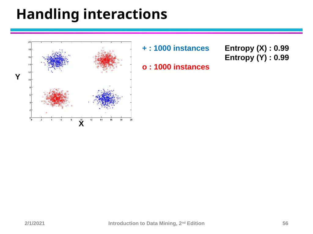
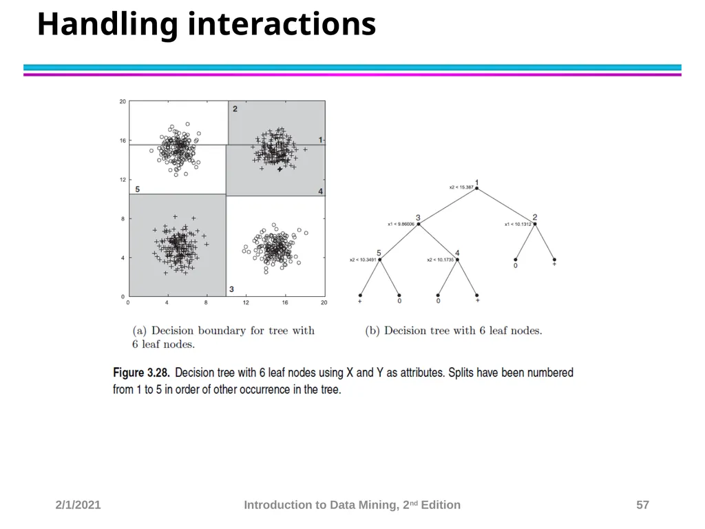
Due to the greedy nature of splitting criterion, interacting attributes (that can distinguish between classes together but not individually) may be passed over in favor of other attributed that are less discriminating.
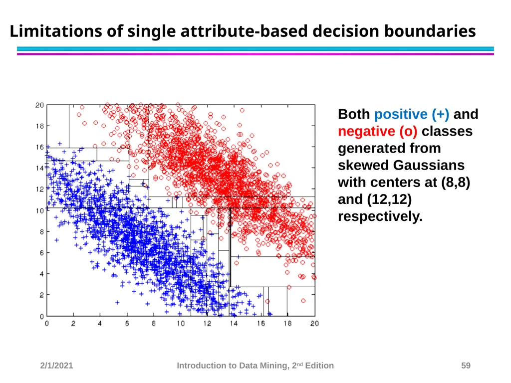
Each decision boundary involves only a single attribute 2/1/2021 Introduction to Data Mining, 2nd Edition 55<br>
Relatively inexpensive to construct
Extremely fast at classifying unknown records
Easy to interpret for small-sized trees
Robust to noise (especially when methods to avoid overfitting are employed)
Can easily handle redundant attributes
Can easily handle irrelevant attributes (unless the attributes are interacting)
Disadvantages: .
Due to the greedy nature of splitting criterion, interacting attributes (that can distinguish between classes together but not individually) may be passed over in favor of other attributed that are less discriminating.
Each decision boundary involves only a single attribute 2/1/2021 Introduction to Data Mining, 2nd Edition 55<br>
56
Handling interactions X Y + : 1000 instances
o : 1000 instances Entropy (X) : 0.99
Entropy (Y) : 0.99 2/1/2021 Introduction to Data Mining, 2nd Edition 56<br>
o : 1000 instances Entropy (X) : 0.99
Entropy (Y) : 0.99 2/1/2021 Introduction to Data Mining, 2nd Edition 56<br>
57
Handling interactions 2/1/2021 Introduction to Data Mining, 2nd Edition 57<br>
58
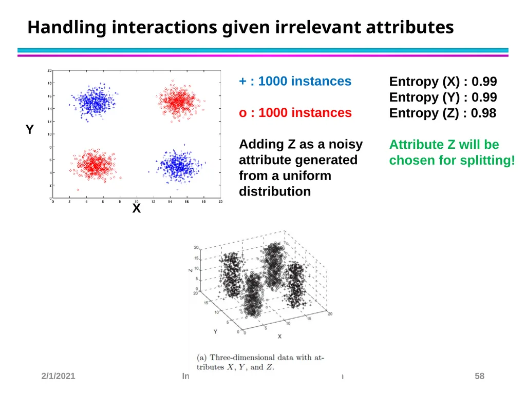
Handling interactions given irrelevant attributes + : 1000 instances
o : 1000 instances
Adding Z as a noisy attribute generated from a uniform distribution Y Entropy (X) : 0.99
Entropy (Y) : 0.99
Entropy (Z) : 0.98
Attribute Z will be chosen for splitting! X 2/1/2021 Introduction to Data Mining, 2nd Edition 58<br>
o : 1000 instances
Adding Z as a noisy attribute generated from a uniform distribution Y Entropy (X) : 0.99
Entropy (Y) : 0.99
Entropy (Z) : 0.98
Attribute Z will be chosen for splitting! X 2/1/2021 Introduction to Data Mining, 2nd Edition 58<br>
59
Limitations of single attribute-based decision boundaries Both positive (+) and negative (o) classes generated from skewed Gaussians with centers at (8,8) and (12,12) respectively. 2/1/2021 Introduction to Data Mining, 2nd Edition 59<br>