
Data Structures Lecture 9 Fang Yu Department of
LS
Published · 47 slides · 0 views

1 / 1
Description
Data Structures Lecture 9 Fang Yu Department of Management Information Systems National Chengchi University Fall 2010 Fundamental Algorithms Divide and Conquer: Merge-sort, Quick-sort, and Recurrence Analysis Divide-and-Conquer A general
Related Topics
Share
Embed code
Download this presentation From Below
"Data Structures Lecture 9 Fang Yu Department of" is the property of its rightful owner. Permission is granted to download and print the materials on this website for personal, non-commercial use only, and to display it on your personal computer provided you do not modify the materials and that you retain all copyright notices contained in the materials. By downloading content from our website, you accept the terms of this agreement.
Presentation Transcript
01
Data Structures
Lecture 9 Fang Yu
Department of Management Information Systems
National Chengchi University Fall 2010<br>
Department of Management Information Systems
National Chengchi University Fall 2010<br>
02
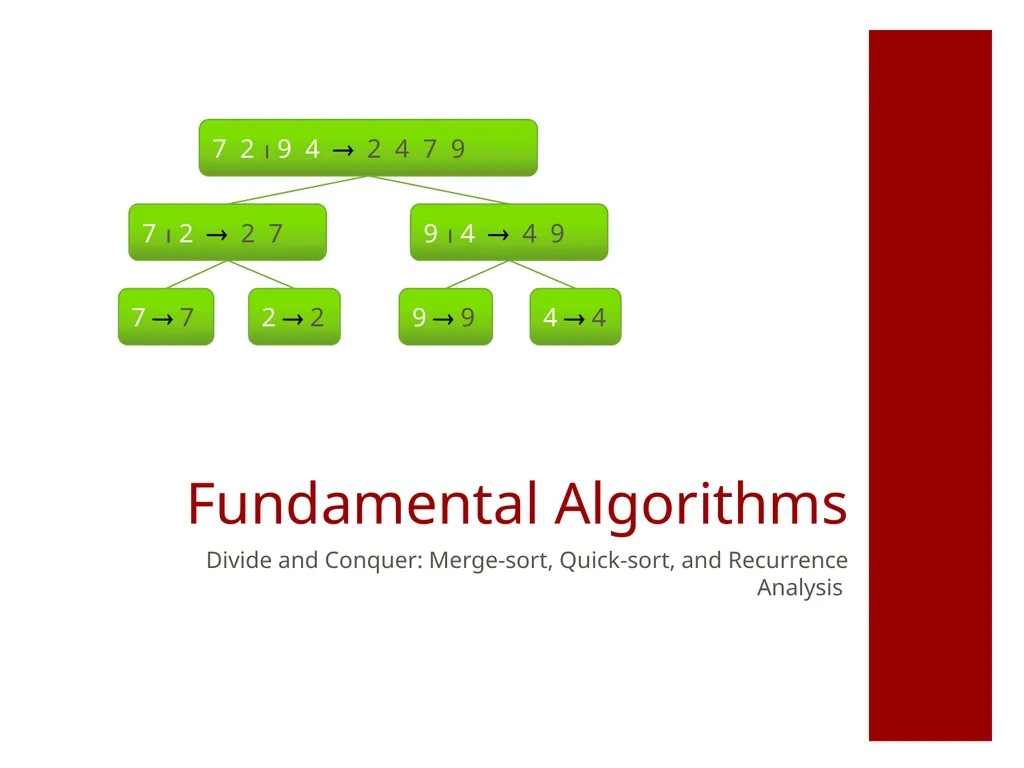
Fundamental Algorithms Divide and Conquer: Merge-sort, Quick-sort, and Recurrence Analysis<br>
03
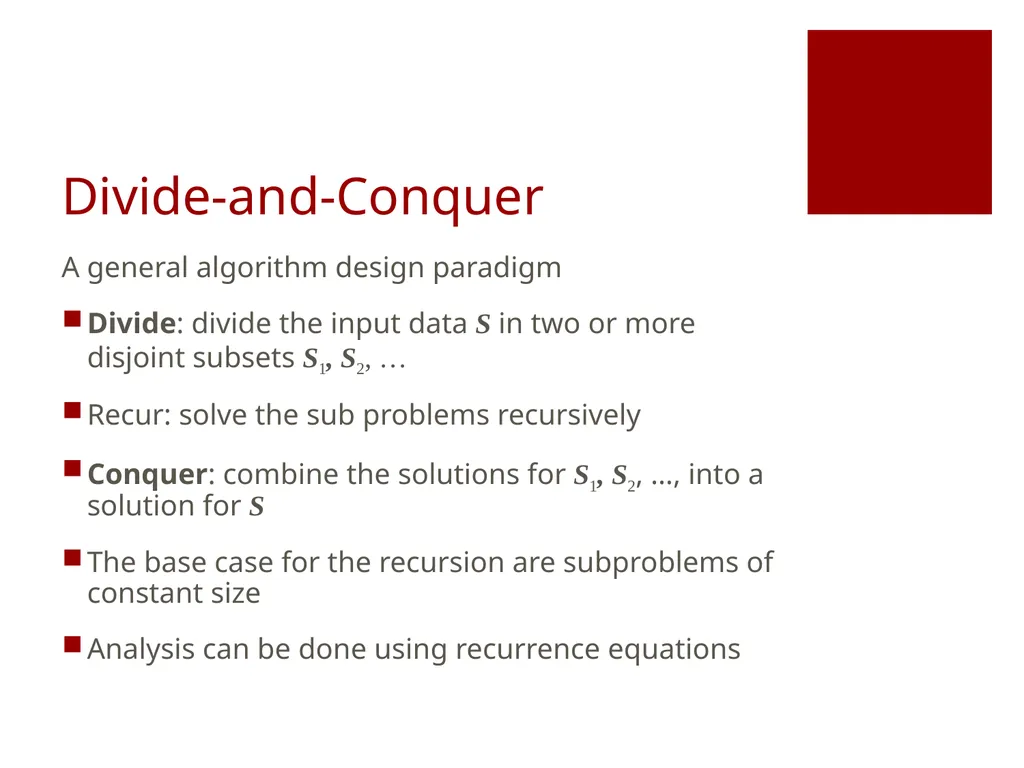
Divide-and-Conquer A general algorithm design paradigm
Divide: divide the input data S in two or more disjoint subsets S1, S2, …
Recur: solve the sub problems recursively
Conquer: combine the solutions for S1, S2, …, into a solution for S
The base case for the recursion are subproblems of constant size
Analysis can be done using recurrence equations<br>
Divide: divide the input data S in two or more disjoint subsets S1, S2, …
Recur: solve the sub problems recursively
Conquer: combine the solutions for S1, S2, …, into a solution for S
The base case for the recursion are subproblems of constant size
Analysis can be done using recurrence equations<br>
04
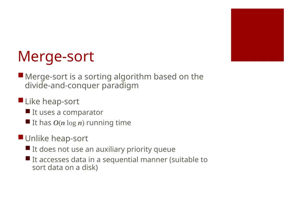
Merge-sort Merge-sort is a sorting algorithm based on the divide-and-conquer paradigm
Like heap-sort
It uses a comparator
It has O(n log n) running time
Unlike heap-sort
It does not use an auxiliary priority queue
It accesses data in a sequential manner (suitable to sort data on a disk)<br>
Like heap-sort
It uses a comparator
It has O(n log n) running time
Unlike heap-sort
It does not use an auxiliary priority queue
It accesses data in a sequential manner (suitable to sort data on a disk)<br>
05
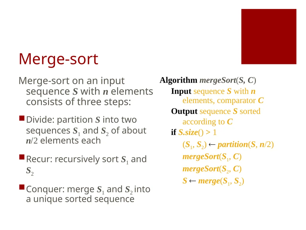
Merge-sort Merge-sort on an input sequence S with n elements consists of three steps:
Divide: partition S into two sequences S1 and S2 of about n/2 elements each
Recur: recursively sort S1 and S2
Conquer: merge S1 and S2 into a unique sorted sequence Algorithm mergeSort(S, C)
Input sequence S with n elements, comparator C
Output sequence S sorted
according to C
if S.size() > 1
(S1, S2) partition(S, n/2)
mergeSort(S1, C)
mergeSort(S2, C)
S merge(S1, S2)<br>
Divide: partition S into two sequences S1 and S2 of about n/2 elements each
Recur: recursively sort S1 and S2
Conquer: merge S1 and S2 into a unique sorted sequence Algorithm mergeSort(S, C)
Input sequence S with n elements, comparator C
Output sequence S sorted
according to C
if S.size() > 1
(S1, S2) partition(S, n/2)
mergeSort(S1, C)
mergeSort(S2, C)
S merge(S1, S2)<br>
06
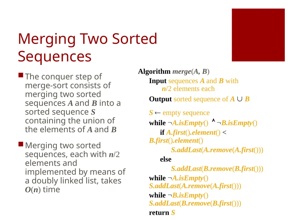
Merging Two Sorted Sequences The conquer step of merge-sort consists of merging two sorted sequences A and B into a sorted sequence S containing the union of the elements of A and B
Merging two sorted sequences, each with n/2 elements and implemented by means of a doubly linked list, takes O(n) time Algorithm merge(A, B)
Input sequences A and B with n/2 elements each
Output sorted sequence of A B
S empty sequence
while A.isEmpty() B.isEmpty()
if A.first().element() < B.first().element()
S.addLast(A.remove(A.first()))
else
S.addLast(B.remove(B.first()))
while A.isEmpty() S.addLast(A.remove(A.first()))
while B.isEmpty() S.addLast(B.remove(B.first()))
return S<br>
Merging two sorted sequences, each with n/2 elements and implemented by means of a doubly linked list, takes O(n) time Algorithm merge(A, B)
Input sequences A and B with n/2 elements each
Output sorted sequence of A B
S empty sequence
while A.isEmpty() B.isEmpty()
if A.first().element() < B.first().element()
S.addLast(A.remove(A.first()))
else
S.addLast(B.remove(B.first()))
while A.isEmpty() S.addLast(A.remove(A.first()))
while B.isEmpty() S.addLast(B.remove(B.first()))
return S<br>
07
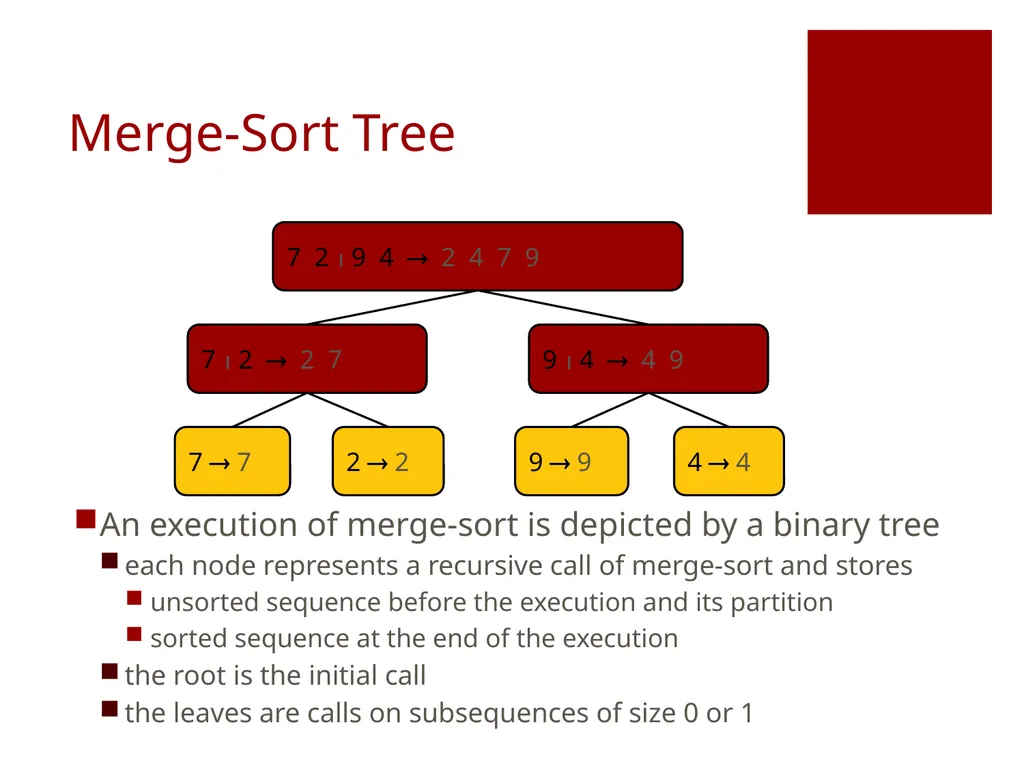
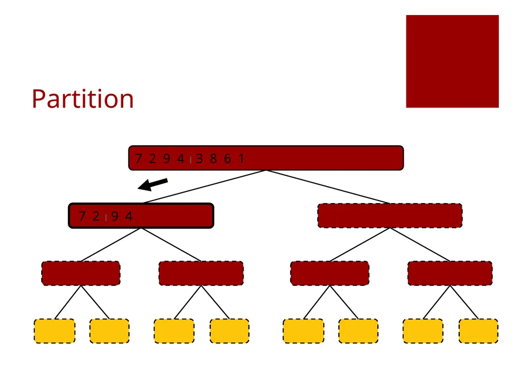
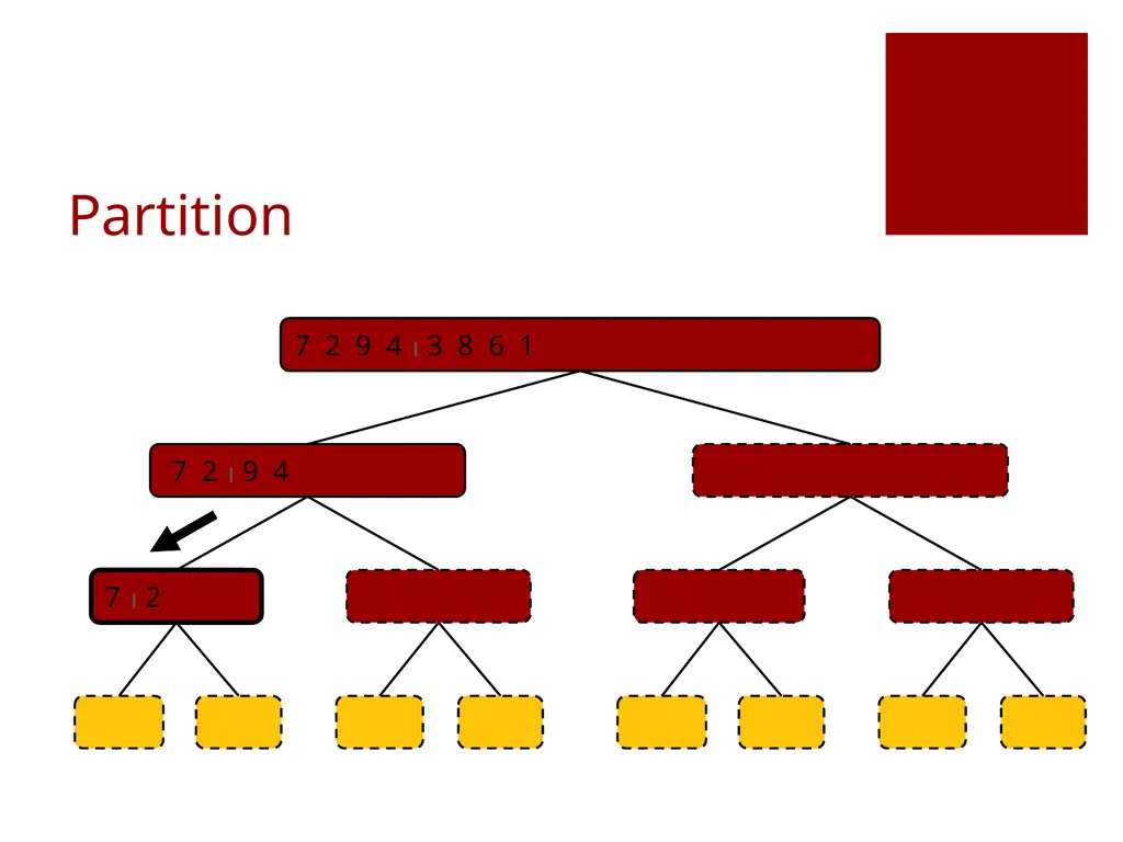
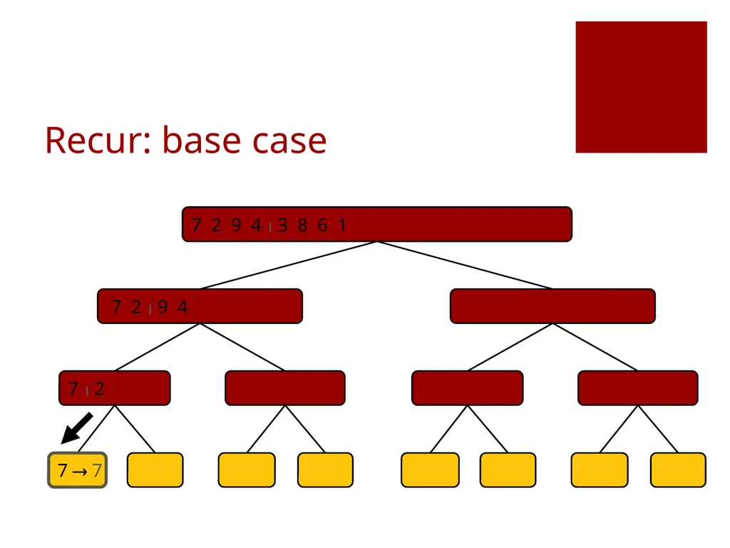
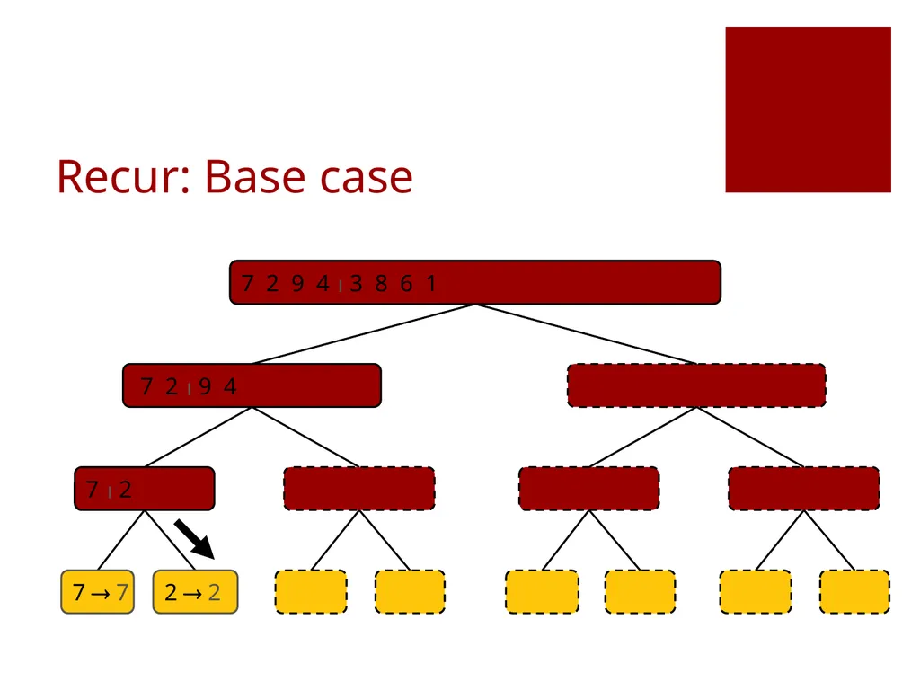
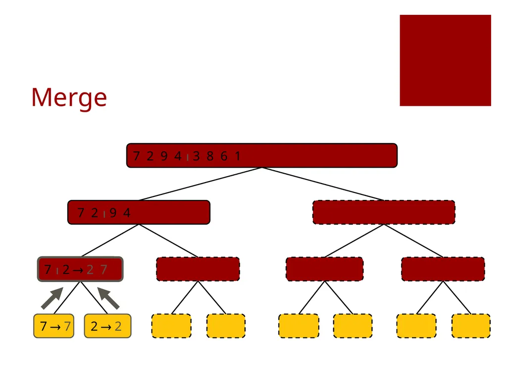
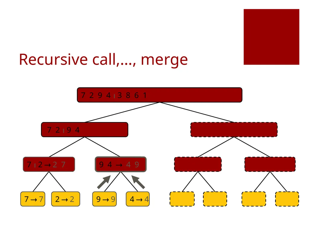
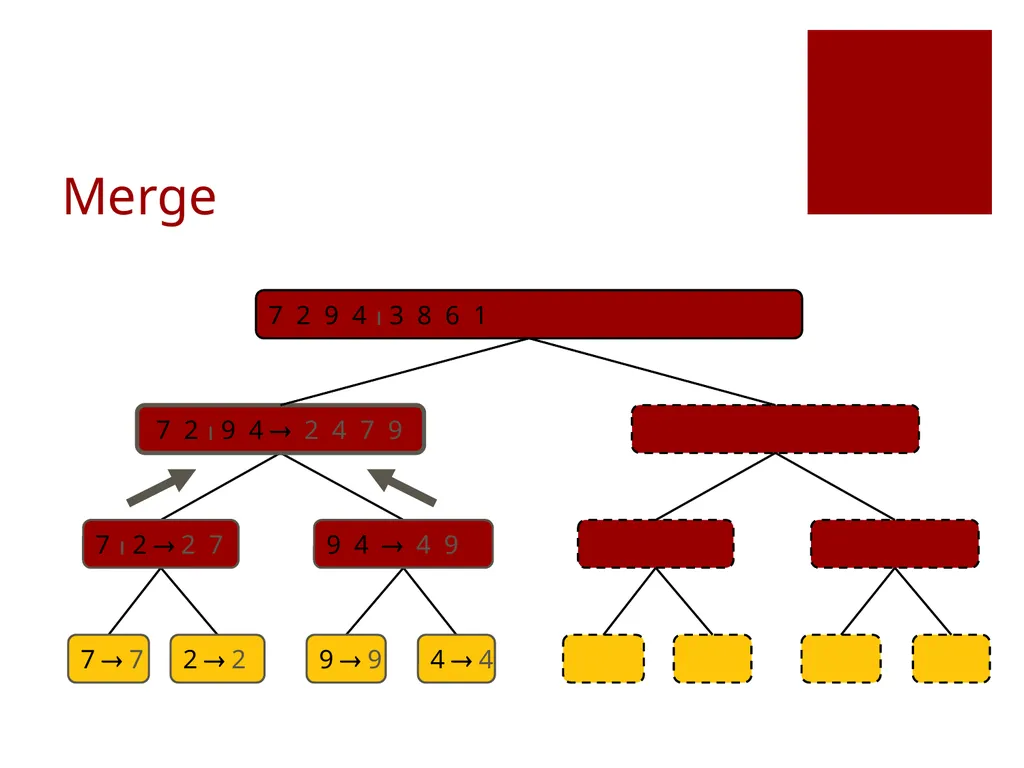
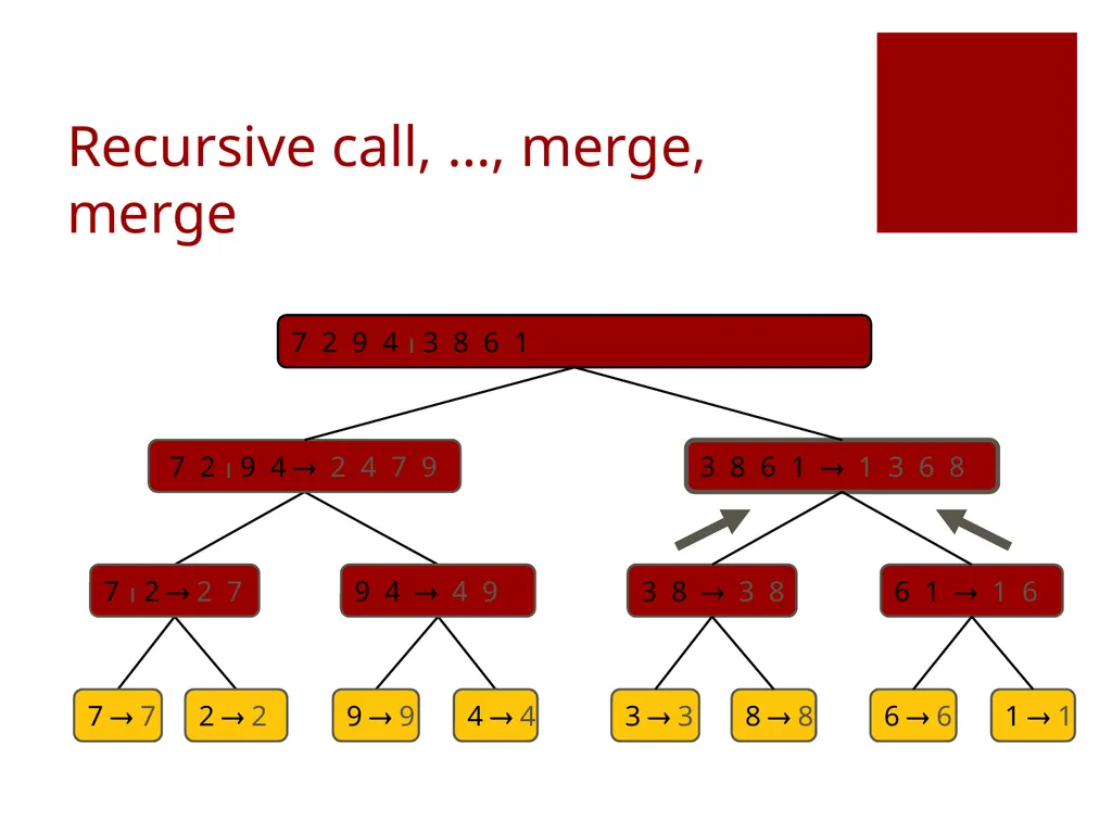
Merge-Sort Tree An execution of merge-sort is depicted by a binary tree
each node represents a recursive call of merge-sort and stores
unsorted sequence before the execution and its partition
sorted sequence at the end of the execution
the root is the initial call
the leaves are calls on subsequences of size 0 or 1 7 2 9 4 2 4 7 9 7 2 2 7 9 4 4 9 7 7 2 2 9 9 4 4<br>
each node represents a recursive call of merge-sort and stores
unsorted sequence before the execution and its partition
sorted sequence at the end of the execution
the root is the initial call
the leaves are calls on subsequences of size 0 or 1 7 2 9 4 2 4 7 9 7 2 2 7 9 4 4 9 7 7 2 2 9 9 4 4<br>
08
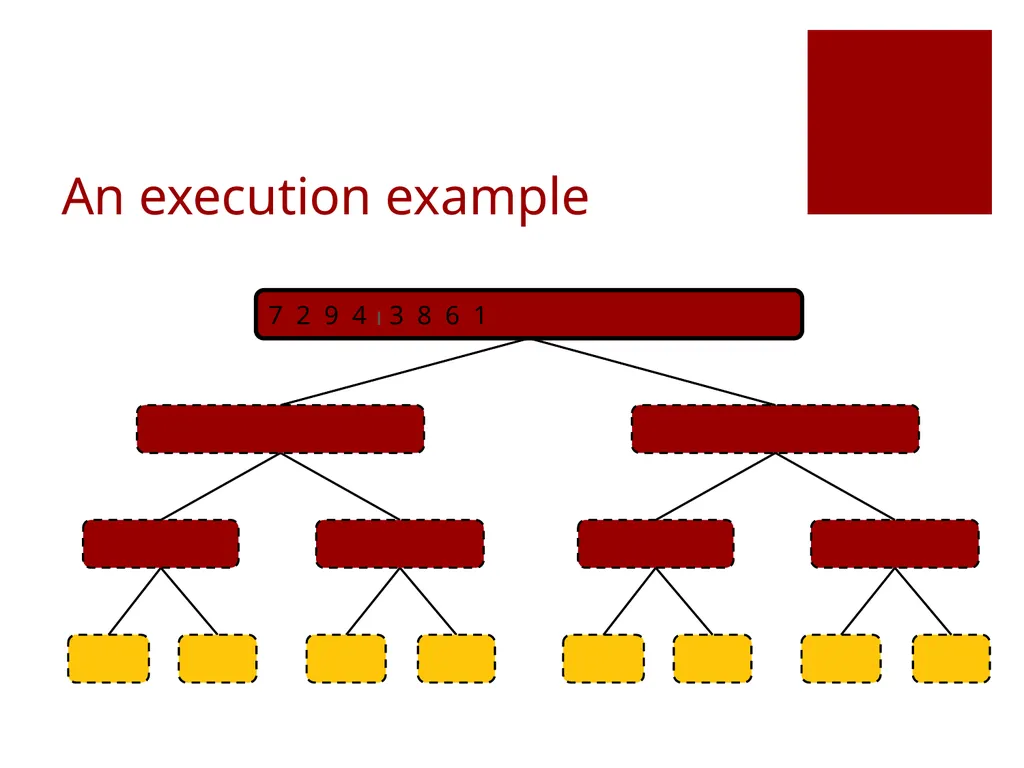
An execution example 7 2 9 4 3 8 6 1 1 2 3 4 6 7 8 9<br>
09
Partition 7 2 9 4 2 4 7 9 3 8 6 1 1 3 8 6 7 2 9 4 3 8 6 1 1 2 3 4 6 7 8 9<br>
10
Partition 7 2 9 4 2 4 7 9 3 8 6 1 1 3 8 6 7 2 2 7 9 4 4 9 3 8 3 8 6 1 1 6 7 2 9 4 3 8 6 1 1 2 3 4 6 7 8 9<br>
11
Recur: base case 7 2 9 4 2 4 7 9 3 8 6 1 1 3 8 6 7 7 2 2 9 9 4 4 3 3 8 8 6 6 1 1 7 2 9 4 3 8 6 1 1 2 3 4 6 7 8 9<br>
12
Recur: Base case 7 2 9 4 2 4 7 9 3 8 6 1 1 3 8 6 7 2 2 7 9 4 4 9 3 8 3 8 6 1 1 6 7 7 2 2 9 9 4 4 3 3 8 8 6 6 1 1 7 2 9 4 3 8 6 1 1 2 3 4 6 7 8 9<br>
13
Merge 7 2 9 4 2 4 7 9 3 8 6 1 1 3 8 6 7 2 2 7 9 4 4 9 3 8 3 8 6 1 1 6 7 7 2 2 9 9 4 4 3 3 8 8 6 6 1 1 7 2 9 4 3 8 6 1 1 2 3 4 6 7 8 9<br>
14
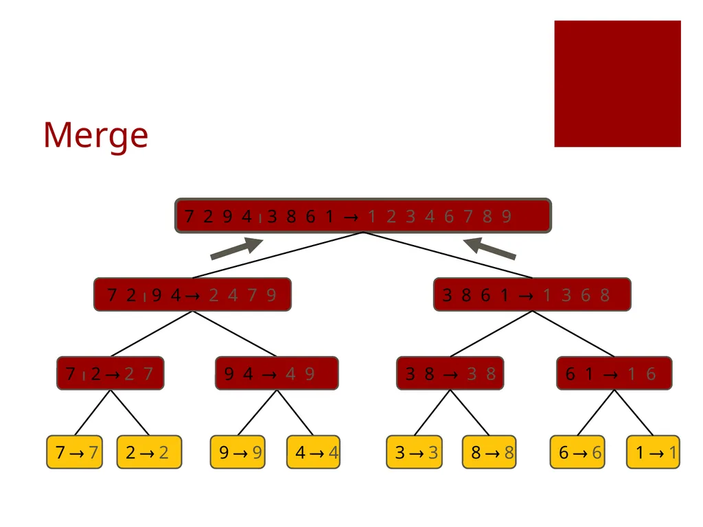
Recursive call,…, merge 7 2 9 4 2 4 7 9 3 8 6 1 1 3 8 6 7 2 2 7 9 4 4 9 3 8 3 8 6 1 1 6 7 7 2 2 3 3 8 8 6 6 1 1 7 2 9 4 3 8 6 1 1 2 3 4 6 7 8 9 9 9 4 4<br>
15
Merge 7 2 9 4 2 4 7 9 3 8 6 1 1 3 8 6 7 2 2 7 9 4 4 9 3 8 3 8 6 1 1 6 7 7 2 2 9 9 4 4 3 3 8 8 6 6 1 1 7 2 9 4 3 8 6 1 1 2 3 4 6 7 8 9<br>
16
Recursive call, …, merge, merge 7 2 9 4 2 4 7 9 3 8 6 1 1 3 6 8 7 2 2 7 9 4 4 9 3 8 3 8 6 1 1 6 7 7 2 2 9 9 4 4 3 3 8 8 6 6 1 1 7 2 9 4 3 8 6 1 1 2 3 4 6 7 8 9<br>
17
Merge 7 2 9 4 2 4 7 9 3 8 6 1 1 3 6 8 7 2 2 7 9 4 4 9 3 8 3 8 6 1 1 6 7 7 2 2 9 9 4 4 3 3 8 8 6 6 1 1 7 2 9 4 3 8 6 1 1 2 3 4 6 7 8 9<br>
18
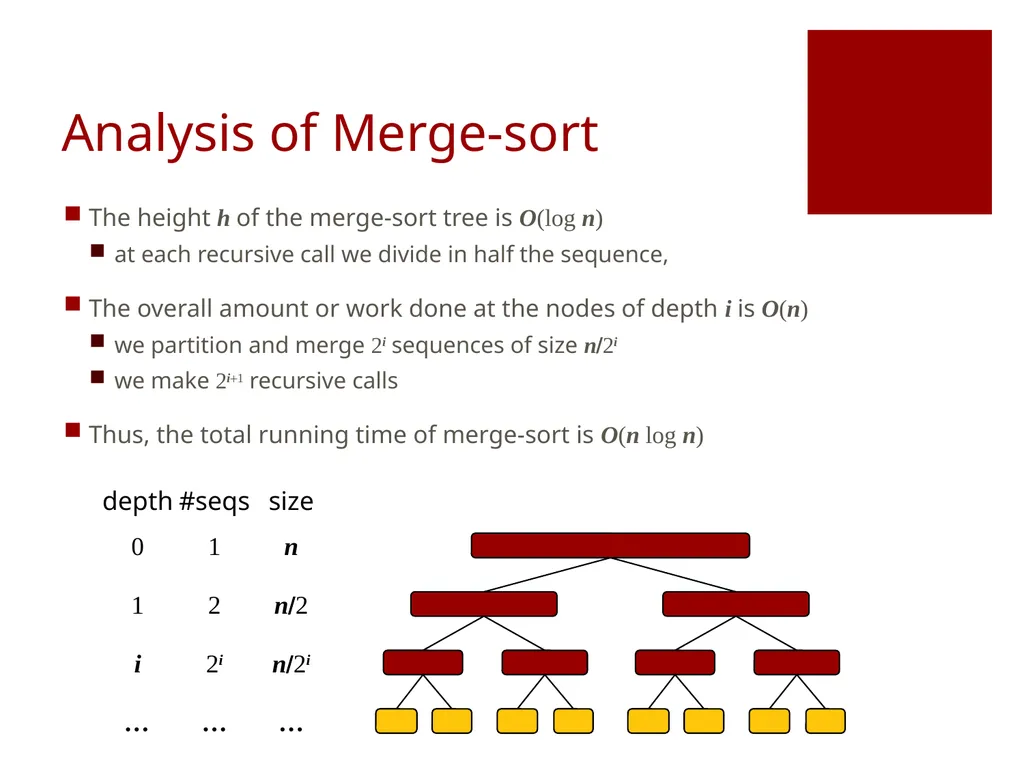
Analysis of Merge-sort The height h of the merge-sort tree is O(log n)
at each recursive call we divide in half the sequence,
The overall amount or work done at the nodes of depth i is O(n)
we partition and merge 2i sequences of size n/2i
we make 2i+1 recursive calls
Thus, the total running time of merge-sort is O(n log n)<br>
at each recursive call we divide in half the sequence,
The overall amount or work done at the nodes of depth i is O(n)
we partition and merge 2i sequences of size n/2i
we make 2i+1 recursive calls
Thus, the total running time of merge-sort is O(n log n)<br>
19
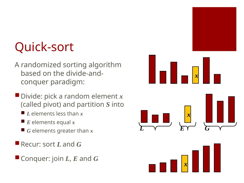
Quick-sort A randomized sorting algorithm based on the divide-and-conquer paradigm:
Divide: pick a random element x (called pivot) and partition S into
L elements less than x
E elements equal x
G elements greater than x
Recur: sort L and G
Conquer: join L, E and G x x L G E x<br>
Divide: pick a random element x (called pivot) and partition S into
L elements less than x
E elements equal x
G elements greater than x
Recur: sort L and G
Conquer: join L, E and G x x L G E x<br>
20
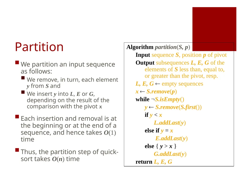
Partition We partition an input sequence as follows:
We remove, in turn, each element y from S and
We insert y into L, E or G, depending on the result of the comparison with the pivot x
Each insertion and removal is at the beginning or at the end of a sequence, and hence takes O(1) time
Thus, the partition step of quick-sort takes O(n) time Algorithm partition(S, p)
Input sequence S, position p of pivot
Output subsequences L, E, G of the elements of S less than, equal to, or greater than the pivot, resp.
L, E, G empty sequences
x S.remove(p)
while S.isEmpty()
y S.remove(S.first())
if y < x
L.addLast(y)
else if y = x
E.addLast(y)
else { y > x }
G.addLast(y)
return L, E, G<br>
We remove, in turn, each element y from S and
We insert y into L, E or G, depending on the result of the comparison with the pivot x
Each insertion and removal is at the beginning or at the end of a sequence, and hence takes O(1) time
Thus, the partition step of quick-sort takes O(n) time Algorithm partition(S, p)
Input sequence S, position p of pivot
Output subsequences L, E, G of the elements of S less than, equal to, or greater than the pivot, resp.
L, E, G empty sequences
x S.remove(p)
while S.isEmpty()
y S.remove(S.first())
if y < x
L.addLast(y)
else if y = x
E.addLast(y)
else { y > x }
G.addLast(y)
return L, E, G<br>
21
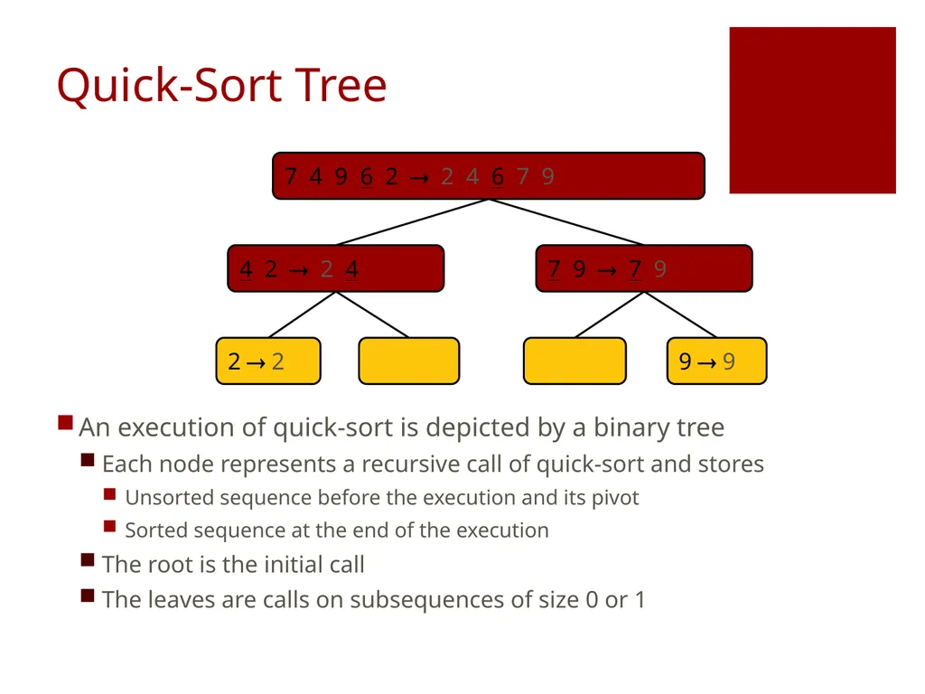
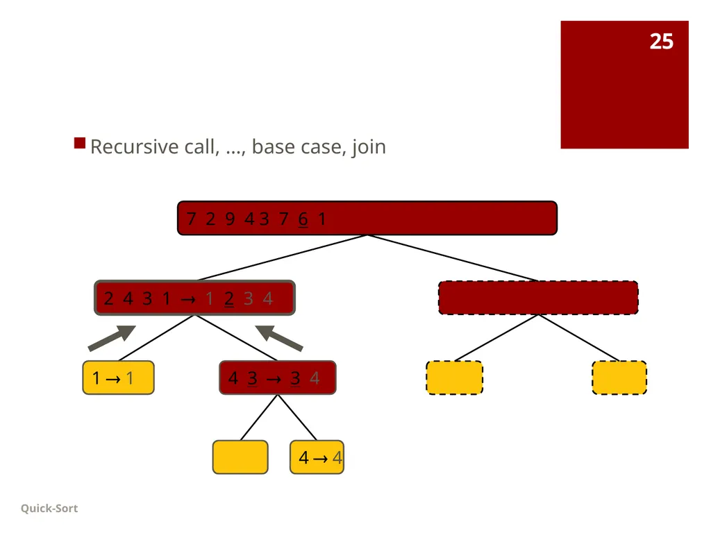
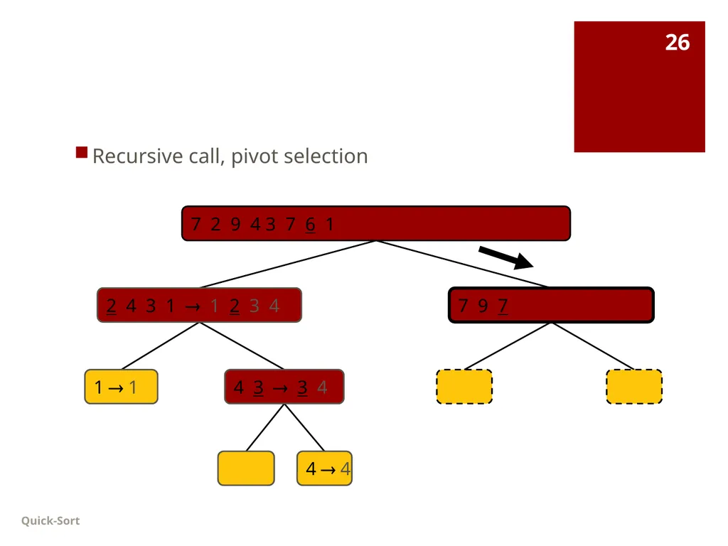
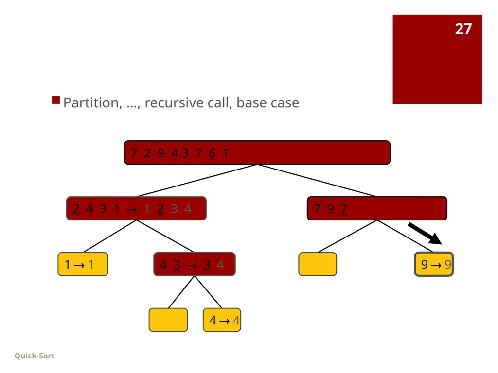
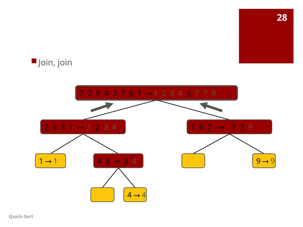
Quick-Sort Tree An execution of quick-sort is depicted by a binary tree
Each node represents a recursive call of quick-sort and stores
Unsorted sequence before the execution and its pivot
Sorted sequence at the end of the execution
The root is the initial call
The leaves are calls on subsequences of size 0 or 1 7 4 9 6 2 2 4 6 7 9 4 2 2 4 7 9 7 9 2 2 9 9<br>
Each node represents a recursive call of quick-sort and stores
Unsorted sequence before the execution and its pivot
Sorted sequence at the end of the execution
The root is the initial call
The leaves are calls on subsequences of size 0 or 1 7 4 9 6 2 2 4 6 7 9 4 2 2 4 7 9 7 9 2 2 9 9<br>
22
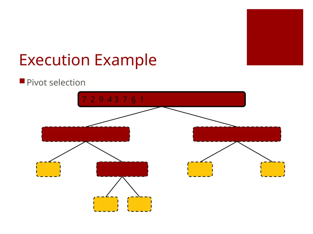
Execution Example Pivot selection 7 2 9 4 2 4 7 9 2 2 7 2 9 4 3 7 6 1 1 2 3 4 6 7 8 9 3 8 6 1 1 3 8 6 3 3 8 8 9 4 4 9 9 9 4 4<br>
23
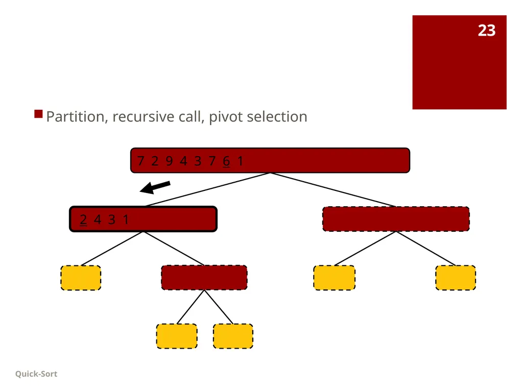
Quick-Sort 23 Partition, recursive call, pivot selection 2 4 3 1 2 4 7 9 9 4 4 9 9 9 4 4 7 2 9 4 3 7 6 1 1 2 3 4 6 7 8 9 3 8 6 1 1 3 8 6 3 3 8 8 2 2<br>
24
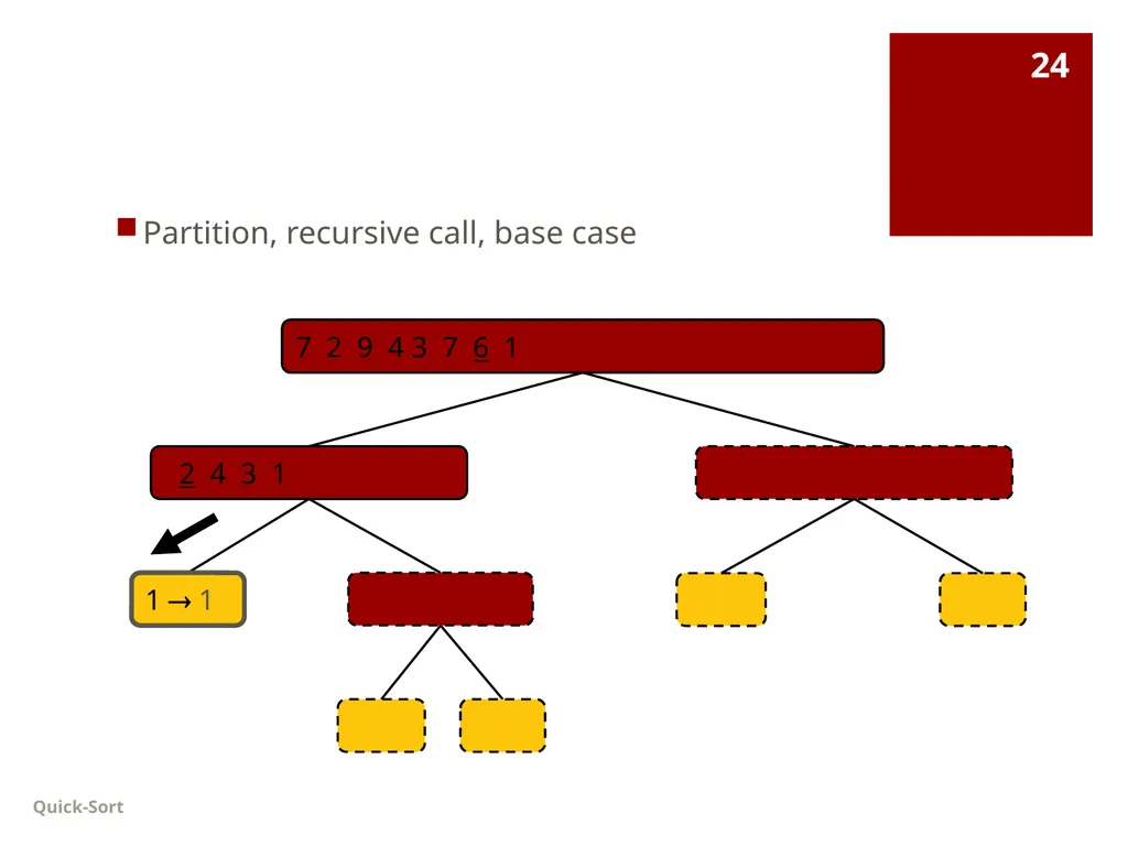
Quick-Sort 24 Partition, recursive call, base case 2 4 3 1 2 4 7 1 1 9 4 4 9 9 9 4 4 7 2 9 4 3 7 6 1 1 2 3 4 6 7 8 9 3 8 6 1 1 3 8 6 3 3 8 8<br>
25
Quick-Sort 25 Recursive call, …, base case, join 3 8 6 1 1 3 8 6 3 3 8 8 7 2 9 4 3 7 6 1 1 2 3 4 6 7 8 9 2 4 3 1 1 2 3 4 1 1 4 3 3 4 9 9 4 4<br>
26
Quick-Sort 26 Recursive call, pivot selection 7 9 7 1 1 3 8 6 8 8 7 2 9 4 3 7 6 1 1 2 3 4 6 7 8 9 2 4 3 1 1 2 3 4 1 1 4 3 3 4 9 9 4 4 9 9<br>
27
Quick-Sort 27 Partition, …, recursive call, base case 7 9 7 1 1 3 8 6 8 8 7 2 9 4 3 7 6 1 1 2 3 4 6 7 8 9 2 4 3 1 1 2 3 4 1 1 4 3 3 4 9 9 4 4 9 9<br>
28
Quick-Sort 28 Join, join 7 9 7 17 7 9 8 8 7 2 9 4 3 7 6 1 1 2 3 4 6 7 7 9 2 4 3 1 1 2 3 4 1 1 4 3 3 4 9 9 4 4 9 9<br>
29
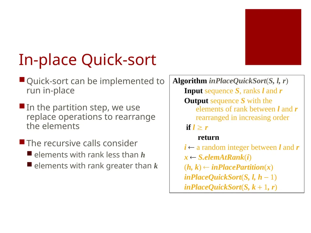
In-place Quick-sort Quick-sort can be implemented to run in-place
In the partition step, we use replace operations to rearrange the elements
The recursive calls consider
elements with rank less than h
elements with rank greater than k Algorithm inPlaceQuickSort(S, l, r)
Input sequence S, ranks l and r
Output sequence S with the elements of rank between l and r rearranged in increasing order
if l r
return
i a random integer between l and r
x S.elemAtRank(i)
(h, k) inPlacePartition(x)
inPlaceQuickSort(S, l, h - 1)
inPlaceQuickSort(S, k + 1, r)<br>
In the partition step, we use replace operations to rearrange the elements
The recursive calls consider
elements with rank less than h
elements with rank greater than k Algorithm inPlaceQuickSort(S, l, r)
Input sequence S, ranks l and r
Output sequence S with the elements of rank between l and r rearranged in increasing order
if l r
return
i a random integer between l and r
x S.elemAtRank(i)
(h, k) inPlacePartition(x)
inPlaceQuickSort(S, l, h - 1)
inPlaceQuickSort(S, k + 1, r)<br>
30
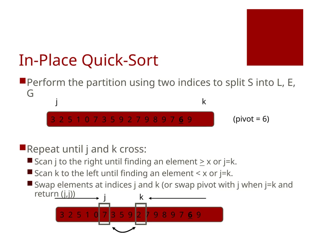
In-Place Quick-Sort Perform the partition using two indices to split S into L, E, G
Repeat until j and k cross:
Scan j to the right until finding an element > x or j=k.
Scan k to the left until finding an element < x or j=k.
Swap elements at indices j and k (or swap pivot with j when j=k and return (j,j)) 3 2 5 1 0 7 3 5 9 2 7 9 8 9 7 6 9 j k (pivot = 6) 3 2 5 1 0 7 3 5 9 2 7 9 8 9 7 6 9 j k<br>
Repeat until j and k cross:
Scan j to the right until finding an element > x or j=k.
Scan k to the left until finding an element < x or j=k.
Swap elements at indices j and k (or swap pivot with j when j=k and return (j,j)) 3 2 5 1 0 7 3 5 9 2 7 9 8 9 7 6 9 j k (pivot = 6) 3 2 5 1 0 7 3 5 9 2 7 9 8 9 7 6 9 j k<br>
31
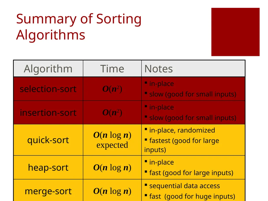
Summary of Sorting Algorithms<br>
32
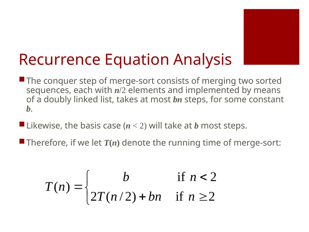
Recurrence Equation Analysis The conquer step of merge-sort consists of merging two sorted sequences, each with n/2 elements and implemented by means of a doubly linked list, takes at most bn steps, for some constant b.
Likewise, the basis case (n < 2) will take at b most steps.
Therefore, if we let T(n) denote the running time of merge-sort:<br>
Likewise, the basis case (n < 2) will take at b most steps.
Therefore, if we let T(n) denote the running time of merge-sort:<br>
33
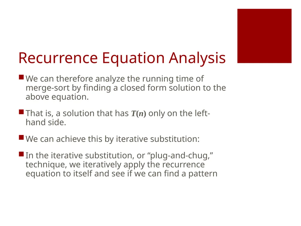
Recurrence Equation Analysis We can therefore analyze the running time of merge-sort by finding a closed form solution to the above equation.
That is, a solution that has T(n) only on the left-hand side.
We can achieve this by iterative substitution:
In the iterative substitution, or “plug-and-chug,” technique, we iteratively apply the recurrence equation to itself and see if we can find a pattern<br>
That is, a solution that has T(n) only on the left-hand side.
We can achieve this by iterative substitution:
In the iterative substitution, or “plug-and-chug,” technique, we iteratively apply the recurrence equation to itself and see if we can find a pattern<br>
34
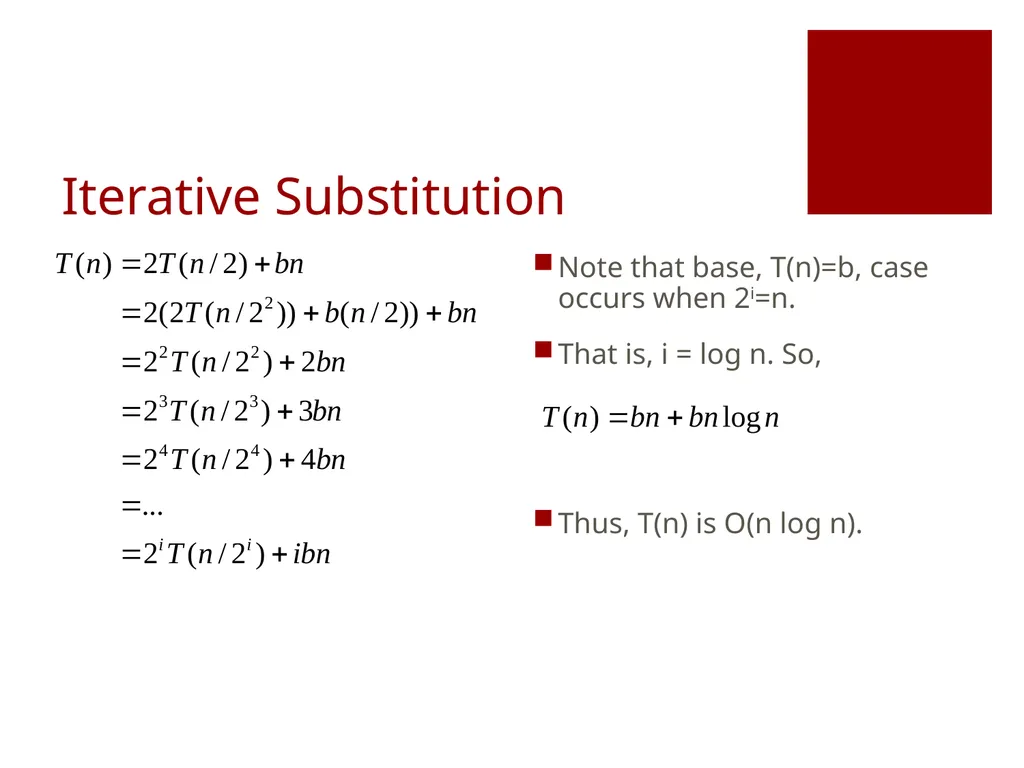
Iterative Substitution Note that base, T(n)=b, case occurs when 2i=n.
That is, i = log n. So,
Thus, T(n) is O(n log n).<br>
That is, i = log n. So,
Thus, T(n) is O(n log n).<br>
35
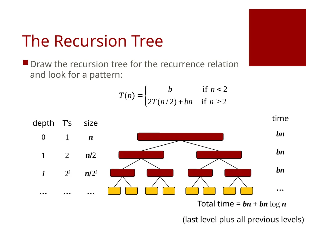
The Recursion Tree Draw the recursion tree for the recurrence relation and look for a pattern: Total time = bn + bn log n (last level plus all previous levels)<br>
36
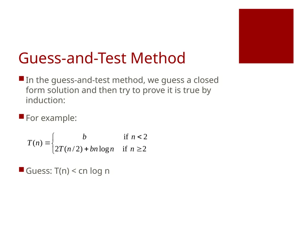
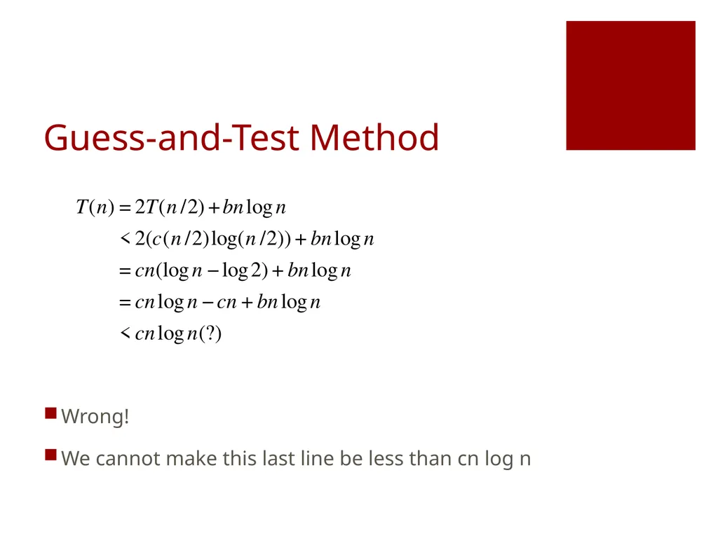
Guess-and-Test Method In the guess-and-test method, we guess a closed form solution and then try to prove it is true by induction:
For example:
Guess: T(n) < cn log n<br>
For example:
Guess: T(n) < cn log n<br>
37
Guess-and-Test Method Wrong!
We cannot make this last line be less than cn log n<br>
We cannot make this last line be less than cn log n<br>
38
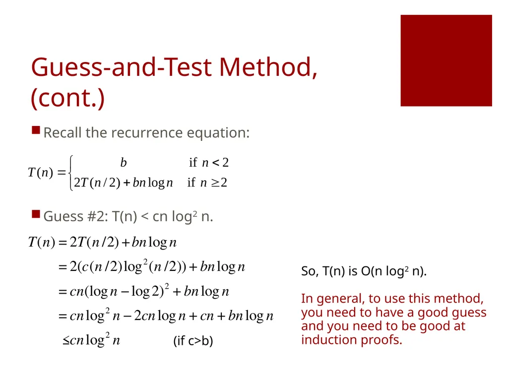
Guess-and-Test Method, (cont.) Recall the recurrence equation:
Guess #2: T(n) < cn log2 n. (if c>b) So, T(n) is O(n log2 n).
In general, to use this method, you need to have a good guess and you need to be good at induction proofs.<br>
Guess #2: T(n) < cn log2 n. (if c>b) So, T(n) is O(n log2 n).
In general, to use this method, you need to have a good guess and you need to be good at induction proofs.<br>
39
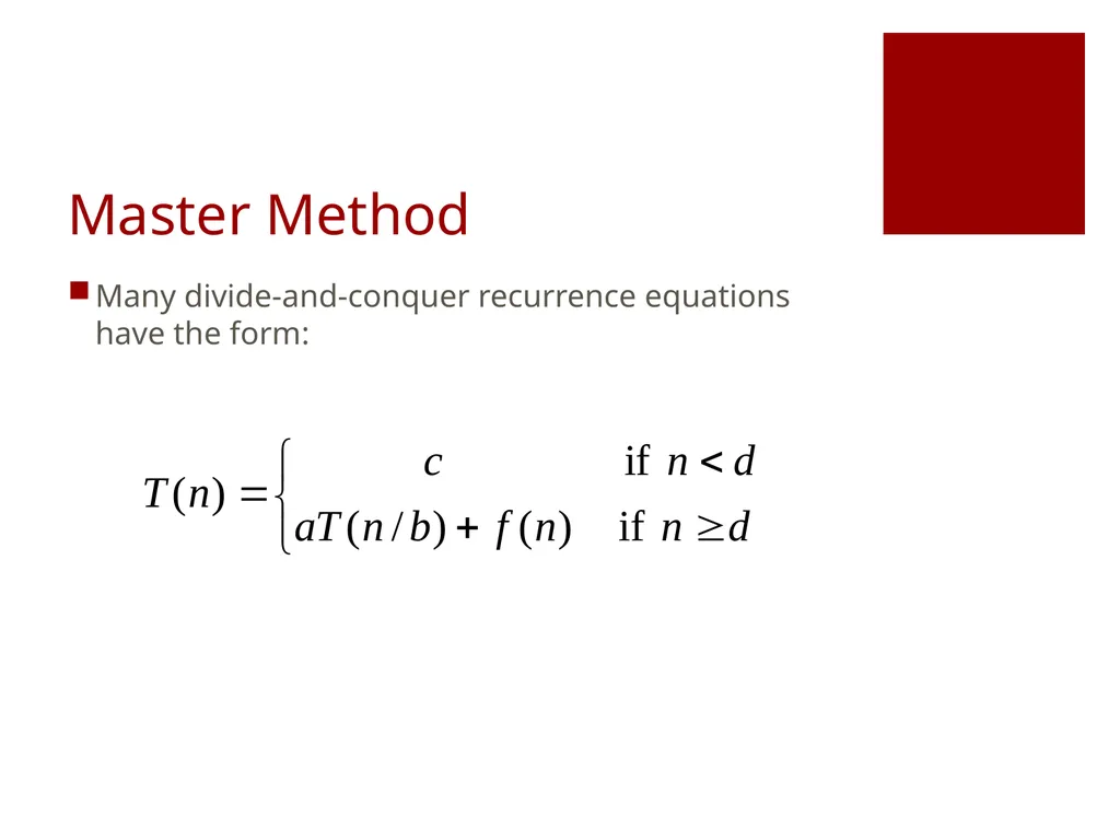
Master Method Many divide-and-conquer recurrence equations have the form:<br>
40
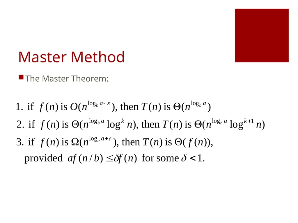
Master Method The Master Theorem:<br>
41
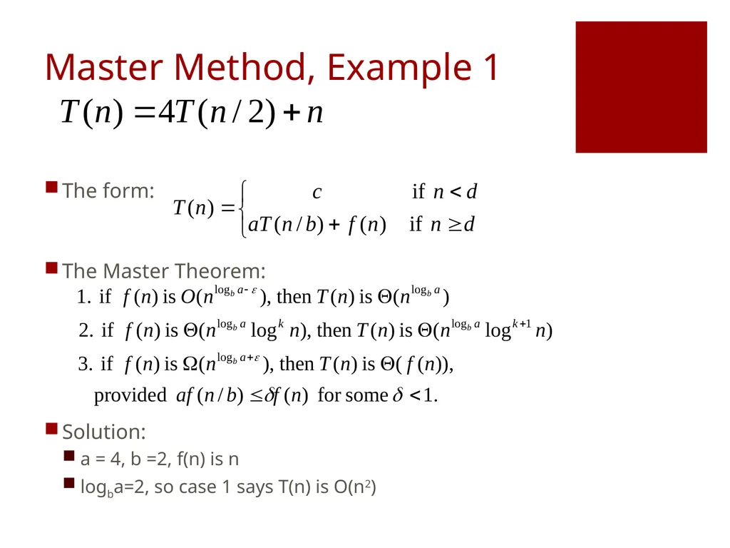
Master Method, Example 1 The form:
The Master Theorem:
Solution:
a = 4, b =2, f(n) is n
logba=2, so case 1 says T(n) is O(n2)<br>
The Master Theorem:
Solution:
a = 4, b =2, f(n) is n
logba=2, so case 1 says T(n) is O(n2)<br>
42
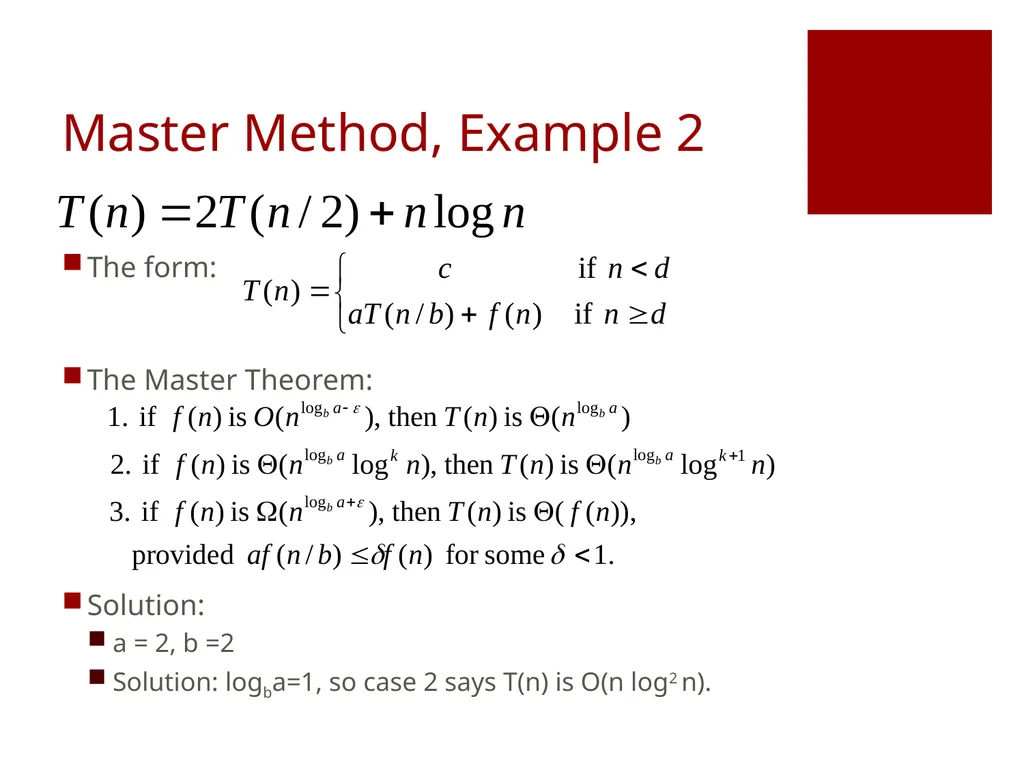
Master Method, Example 2 The form:
The Master Theorem:
Solution:
a = 2, b =2
Solution: logba=1, so case 2 says T(n) is O(n log2 n).<br>
The Master Theorem:
Solution:
a = 2, b =2
Solution: logba=1, so case 2 says T(n) is O(n log2 n).<br>
43
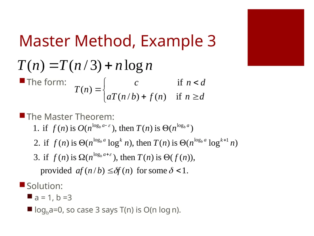
Master Method, Example 3 The form:
The Master Theorem:
Solution:
a = 1, b =3
logba=0, so case 3 says T(n) is O(n log n).<br>
The Master Theorem:
Solution:
a = 1, b =3
logba=0, so case 3 says T(n) is O(n log n).<br>
44
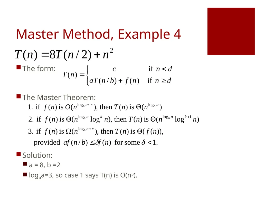
Master Method, Example 4 The form:
The Master Theorem:
Solution:
a = 8, b =2
logba=3, so case 1 says T(n) is O(n3).<br>
The Master Theorem:
Solution:
a = 8, b =2
logba=3, so case 1 says T(n) is O(n3).<br>
45
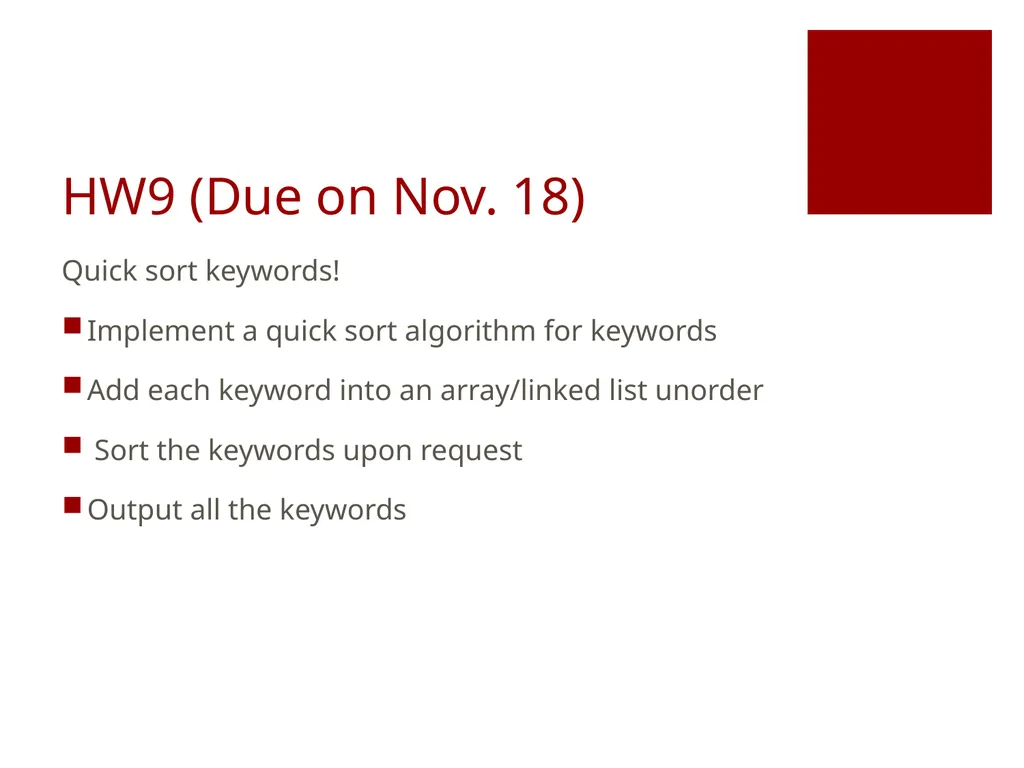
HW9 (Due on Nov. 18) Quick sort keywords!
Implement a quick sort algorithm for keywords
Add each keyword into an array/linked list unorder
Sort the keywords upon request
Output all the keywords<br>
Implement a quick sort algorithm for keywords
Add each keyword into an array/linked list unorder
Sort the keywords upon request
Output all the keywords<br>
46
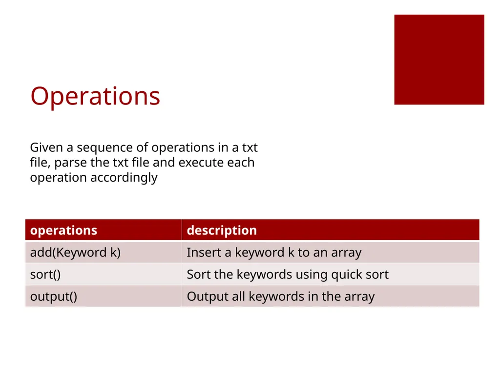
Operations Given a sequence of operations in a txt file, parse the txt file and execute each operation accordingly<br>
47
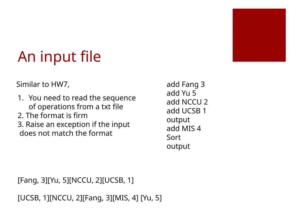
An input file add Fang 3
add Yu 5
add NCCU 2
add UCSB 1
output
add MIS 4
Sort
output You need to read the sequence of operations from a txt file
2. The format is firm
3. Raise an exception if the input
does not match the format Similar to HW7, [Fang, 3][Yu, 5][NCCU, 2][UCSB, 1]
[UCSB, 1][NCCU, 2][Fang, 3][MIS, 4] [Yu, 5]<br>
add Yu 5
add NCCU 2
add UCSB 1
output
add MIS 4
Sort
output You need to read the sequence of operations from a txt file
2. The format is firm
3. Raise an exception if the input
does not match the format Similar to HW7, [Fang, 3][Yu, 5][NCCU, 2][UCSB, 1]
[UCSB, 1][NCCU, 2][Fang, 3][MIS, 4] [Yu, 5]<br>