04
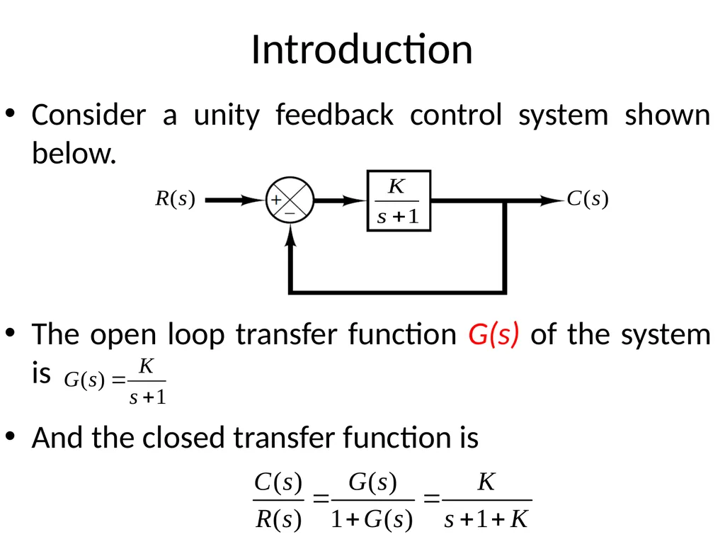
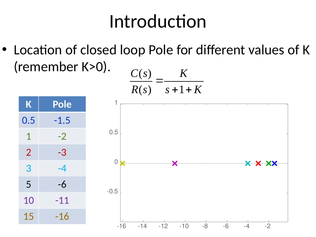
Introduction Location of closed loop Pole for different values of K (remember K>0).<br>
05
What is Root Locus? The root locus is the path of the roots of the characteristic equation traced out in the s-plane as a system parameter varies from zero to infinity.<br>
06
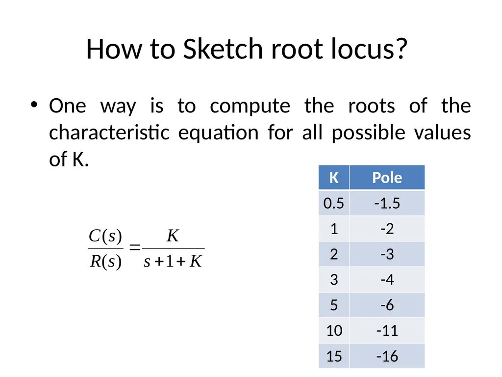
How to Sketch root locus? One way is to compute the roots of the characteristic equation for all possible values of K.<br>
07
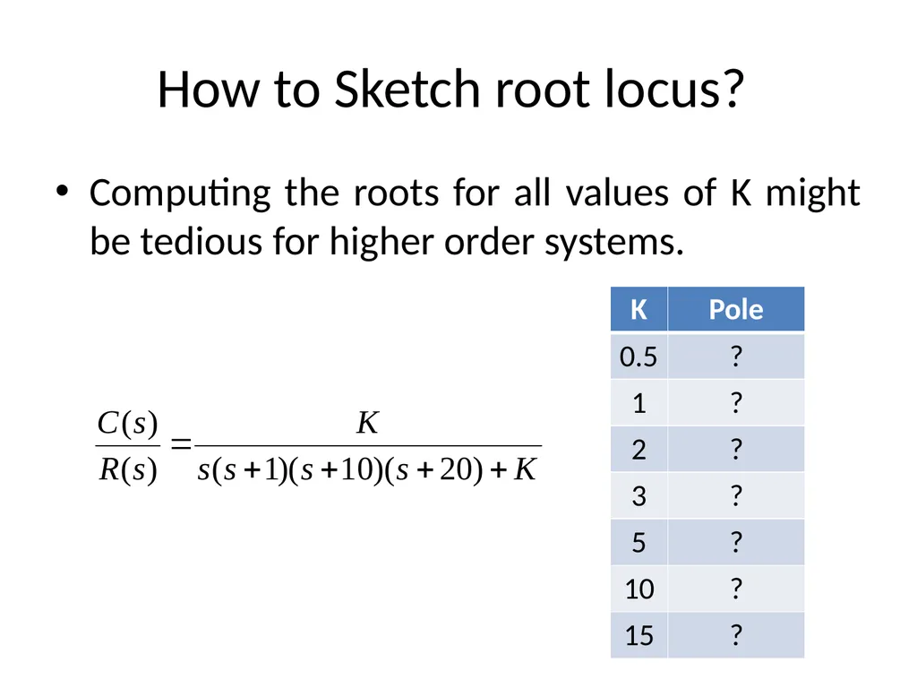
How to Sketch root locus? Computing the roots for all values of K might be tedious for higher order systems.<br>
08
Construction of Root Loci Finding the roots of the characteristic equation of degree higher than 3 is laborious and will need computer solution.
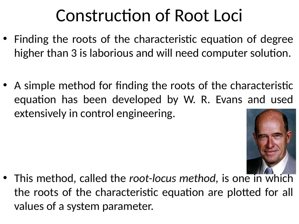
A simple method for finding the roots of the characteristic equation has been developed by W. R. Evans and used extensively in control engineering.
This method, called the root-locus method, is one in which the roots of the characteristic equation are plotted for all values of a system parameter.<br>
09
Construction of Root Loci The roots corresponding to a particular value of this parameter can then be located on the resulting graph.
By using the root-locus method the designer can predict the effects on the location of the closed-loop poles of varying the gain value or adding open-loop poles and/or open-loop zeros.<br>
10
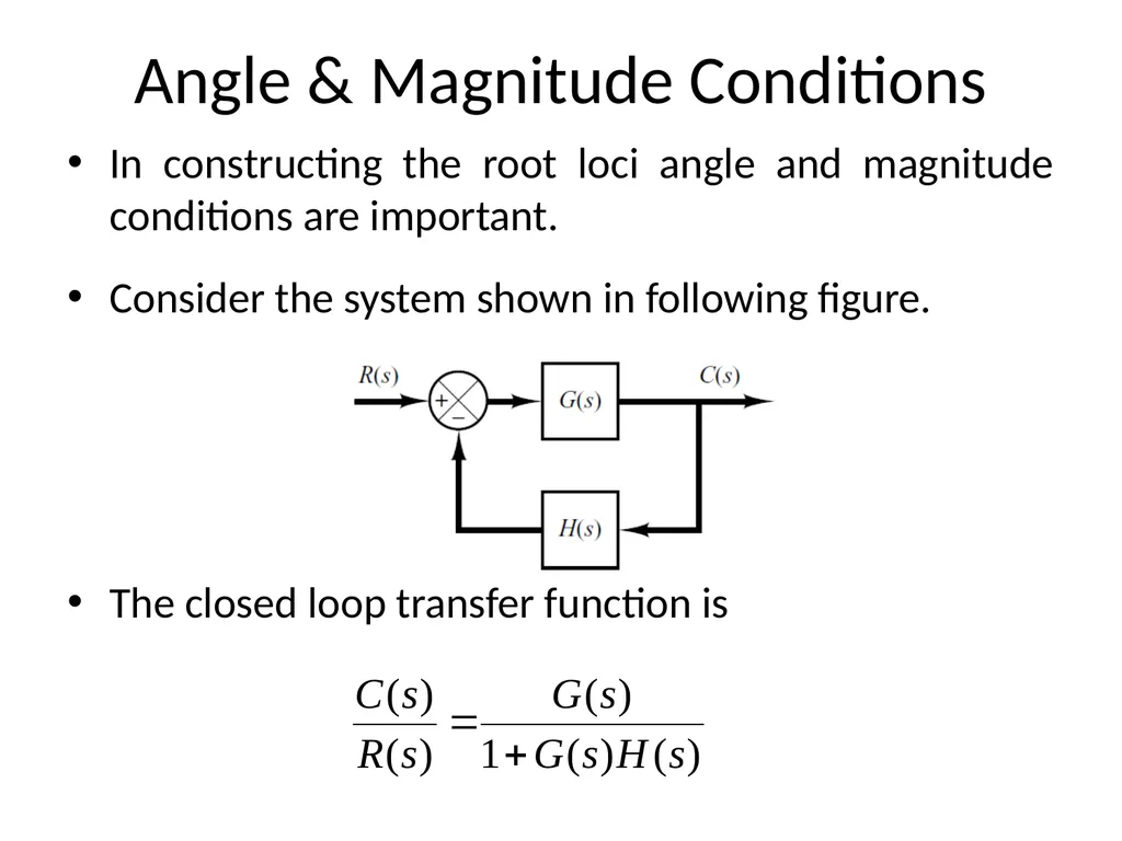
Angle & Magnitude Conditions In constructing the root loci angle and magnitude conditions are important.
Consider the system shown in following figure.
The closed loop transfer function is<br>
11
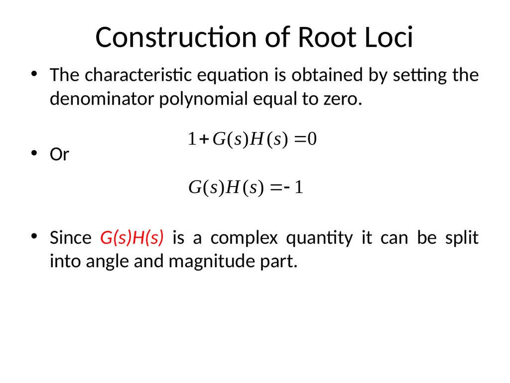
Construction of Root Loci The characteristic equation is obtained by setting the denominator polynomial equal to zero.
Or
Since G(s)H(s) is a complex quantity it can be split into angle and magnitude part.<br>
12
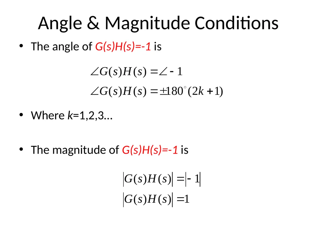
Angle & Magnitude Conditions The angle of G(s)H(s)=-1 is
Where k=1,2,3…
The magnitude of G(s)H(s)=-1 is<br>
13
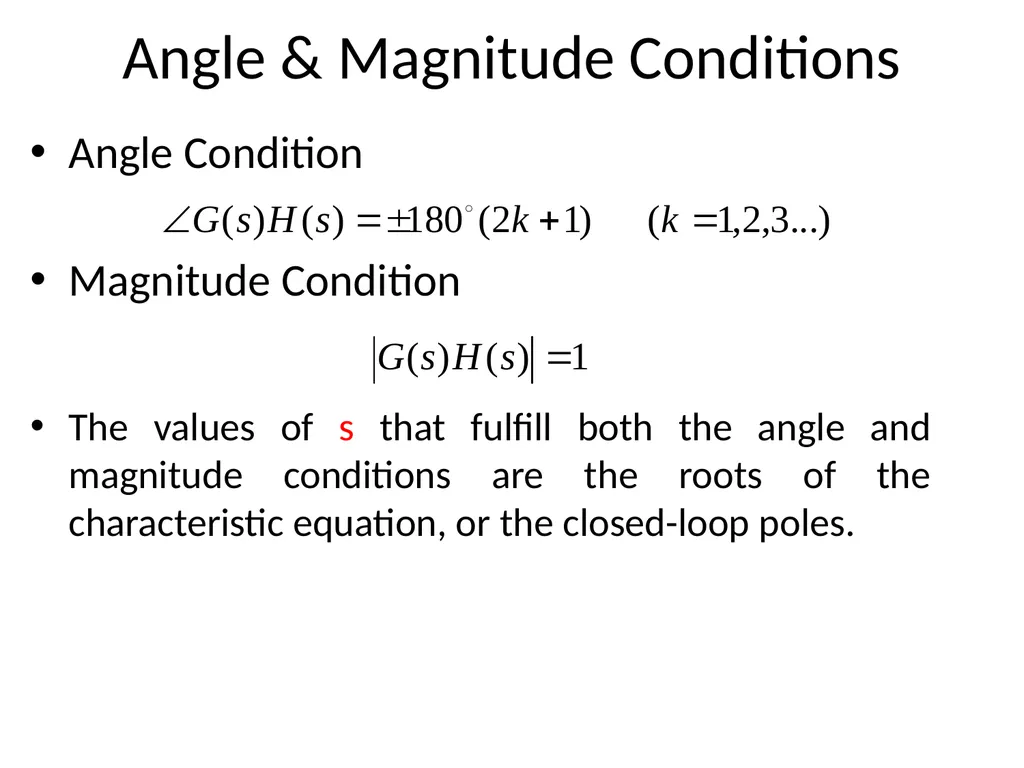
Angle & Magnitude Conditions Angle Condition
Magnitude Condition
The values of s that fulfill both the angle and magnitude conditions are the roots of the characteristic equation, or the closed-loop poles.<br>
14
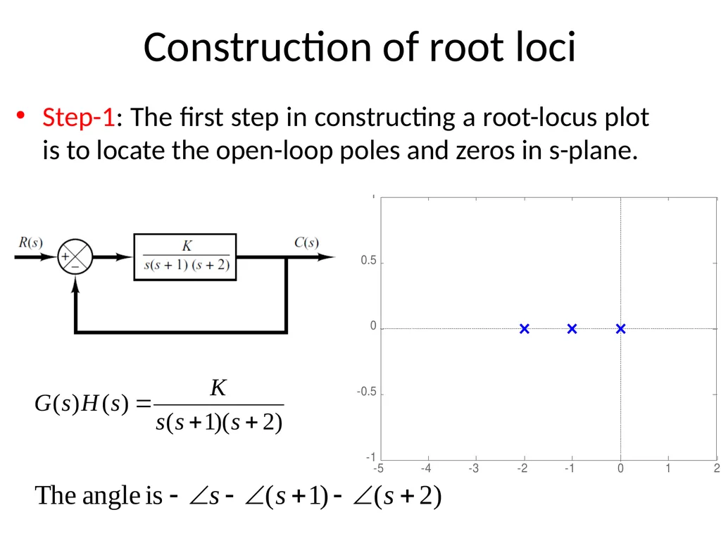
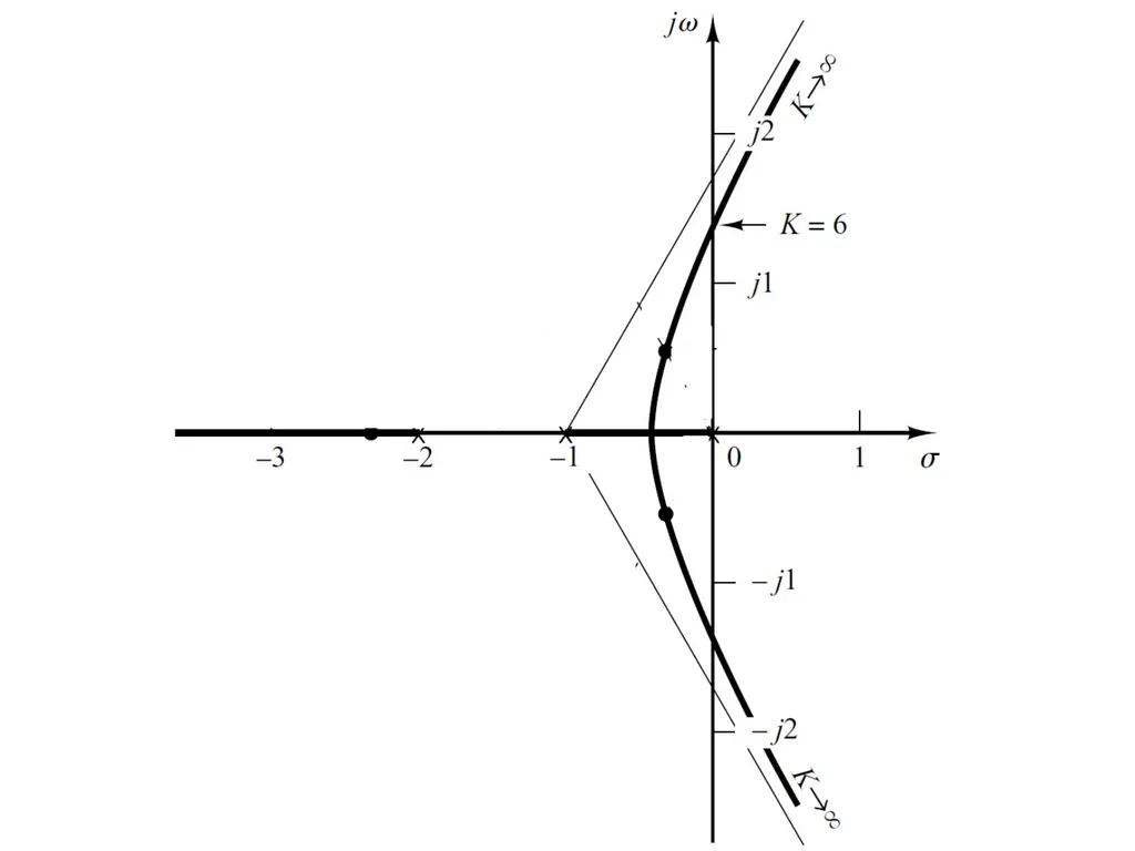
Construction of root loci Step-1: The first step in constructing a root-locus plot is to locate the open-loop poles and zeros in s-plane.<br>
15
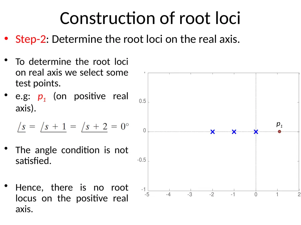
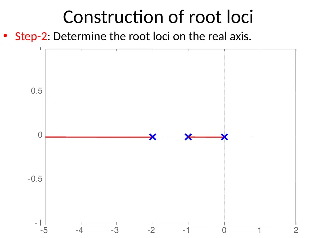
Construction of root loci Step-2: Determine the root loci on the real axis. To determine the root loci on real axis we select some test points.
e.g: p1 (on positive real axis).
The angle condition is not satisfied.
Hence, there is no root locus on the positive real axis.<br>
16
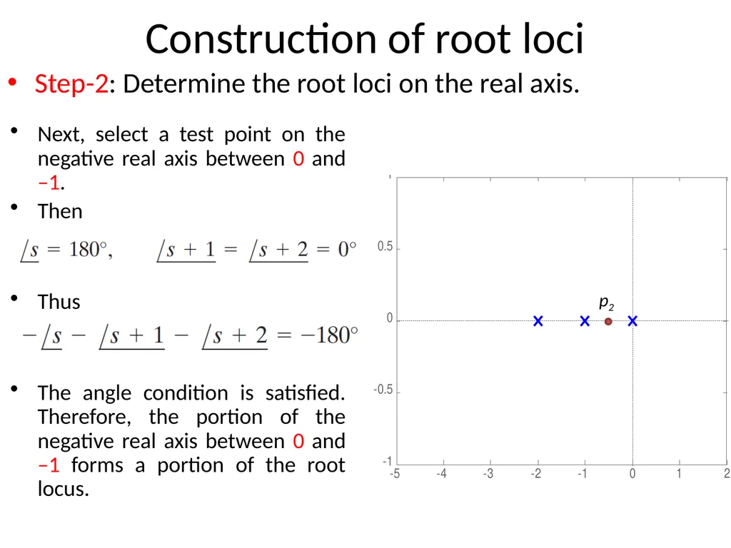
Construction of root loci Step-2: Determine the root loci on the real axis. Next, select a test point on the negative real axis between 0 and –1.
Then
Thus
The angle condition is satisfied. Therefore, the portion of the negative real axis between 0 and –1 forms a portion of the root locus.<br>
17
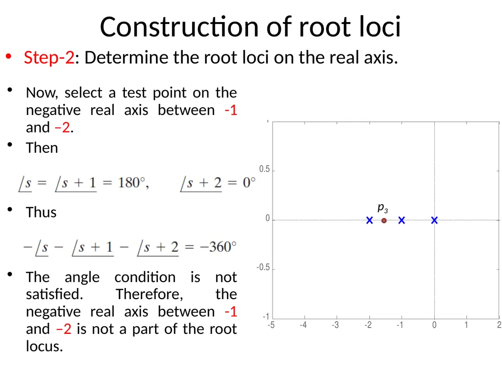
Construction of root loci Step-2: Determine the root loci on the real axis. Now, select a test point on the negative real axis between -1 and –2.
Then
Thus
The angle condition is not satisfied. Therefore, the negative real axis between -1 and –2 is not a part of the root locus.<br>
18
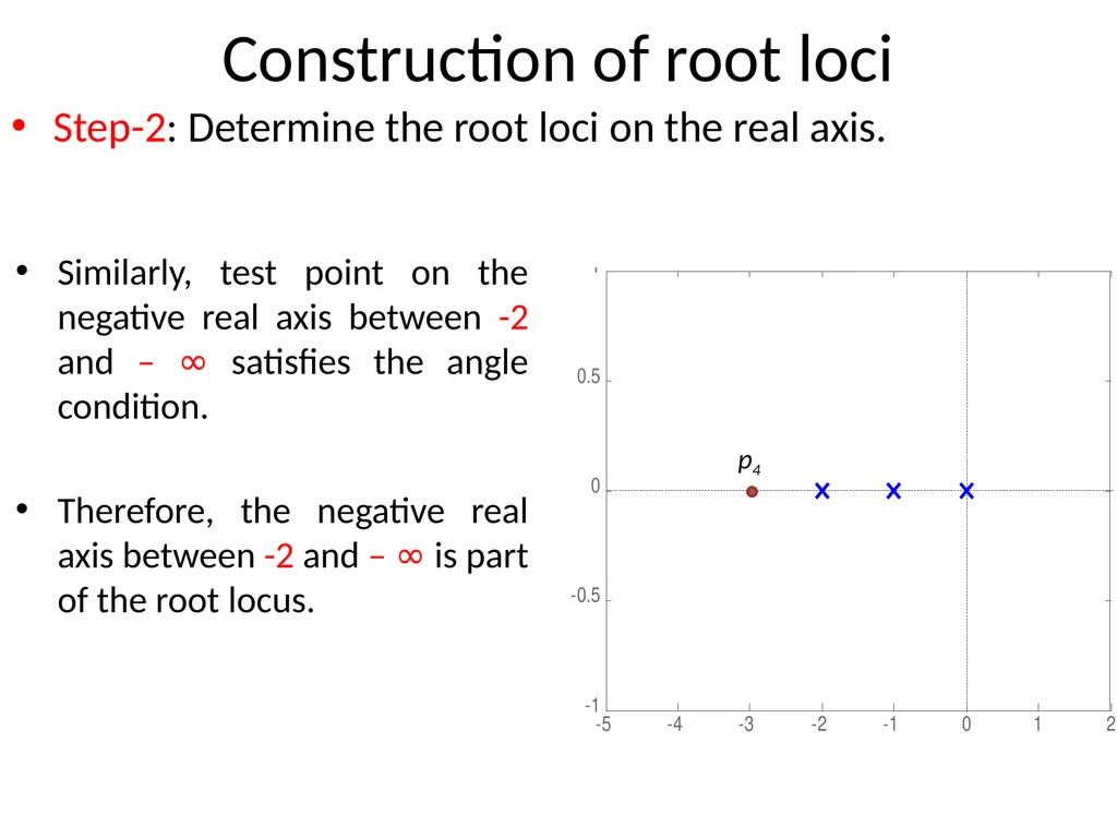
Construction of root loci Step-2: Determine the root loci on the real axis. Similarly, test point on the negative real axis between -2 and – ∞ satisfies the angle condition.
Therefore, the negative real axis between -2 and – ∞ is part of the root locus.<br>
19
Construction of root loci Step-2: Determine the root loci on the real axis.<br>
20
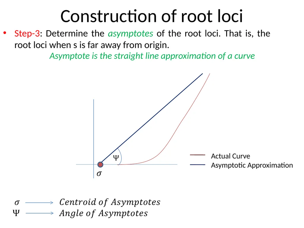
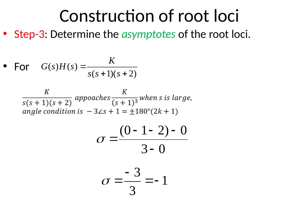
Construction of root loci Step-3: Determine the asymptotes of the root loci. That is, the root loci when s is far away from origin. Asymptote is the straight line approximation of a curve<br>
21
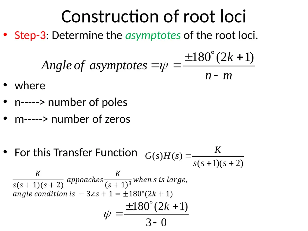
Construction of root loci Step-3: Determine the asymptotes of the root loci.
where
n-----> number of poles
m-----> number of zeros
For this Transfer Function<br>
22
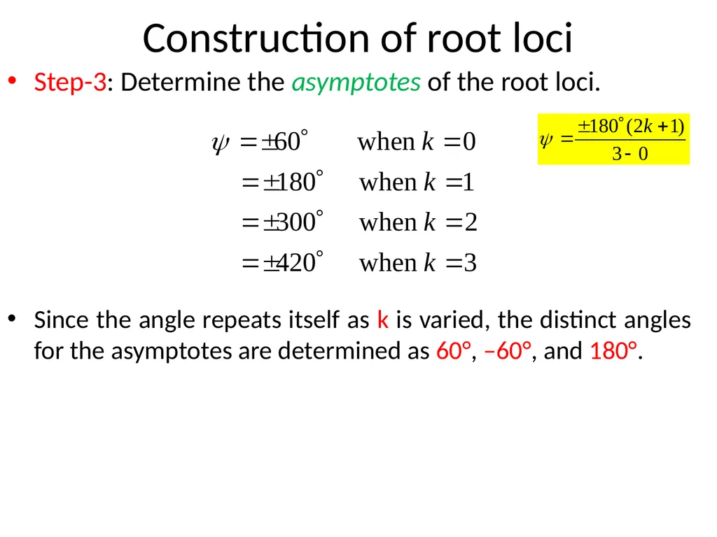
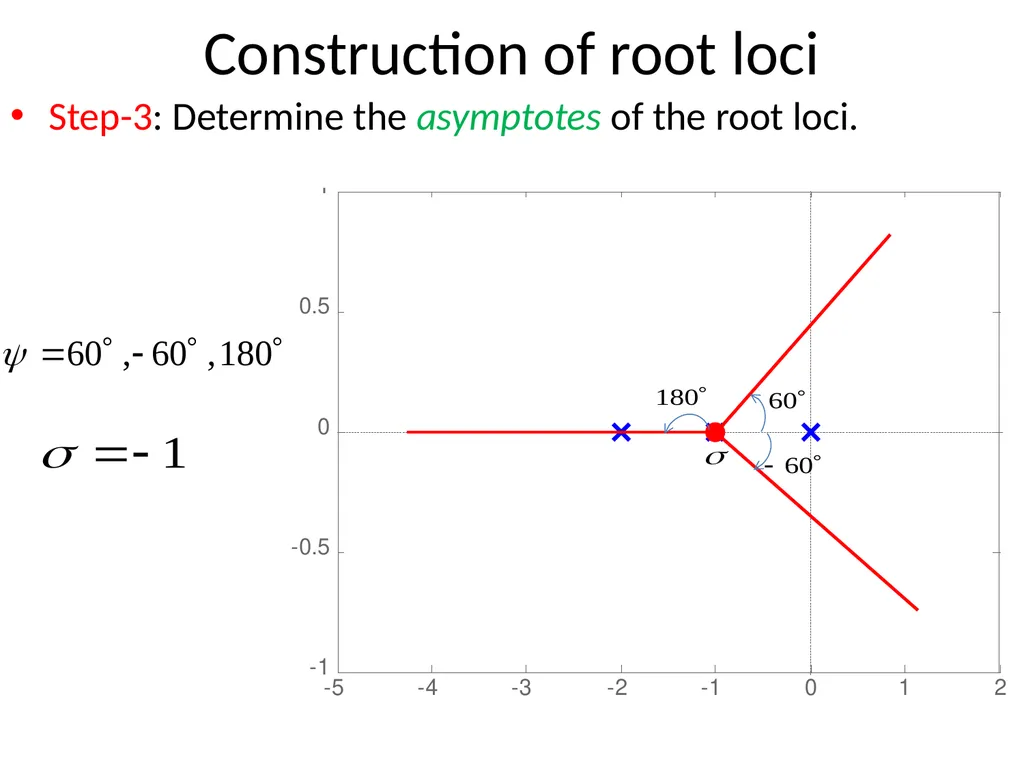
Construction of root loci Step-3: Determine the asymptotes of the root loci.
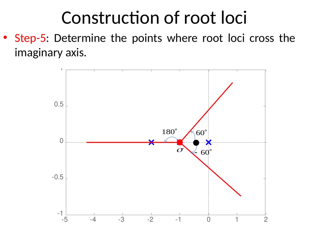
Since the angle repeats itself as k is varied, the distinct angles for the asymptotes are determined as 60°, –60°, and 180°.<br>
23
Construction of root loci Step-3: Determine the asymptotes of the root loci.
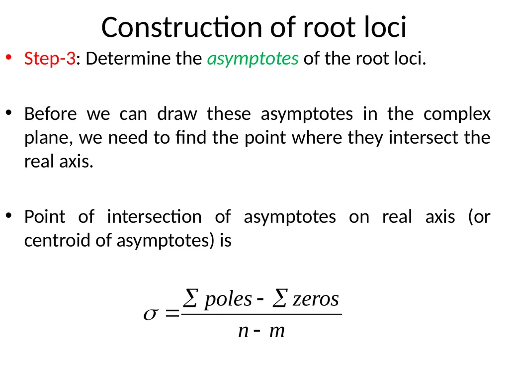
Before we can draw these asymptotes in the complex plane, we need to find the point where they intersect the real axis.
Point of intersection of asymptotes on real axis (or centroid of asymptotes) is<br>
24
Construction of root loci Step-3: Determine the asymptotes of the root loci.
For<br>
25
Construction of root loci Step-3: Determine the asymptotes of the root loci.<br>
26
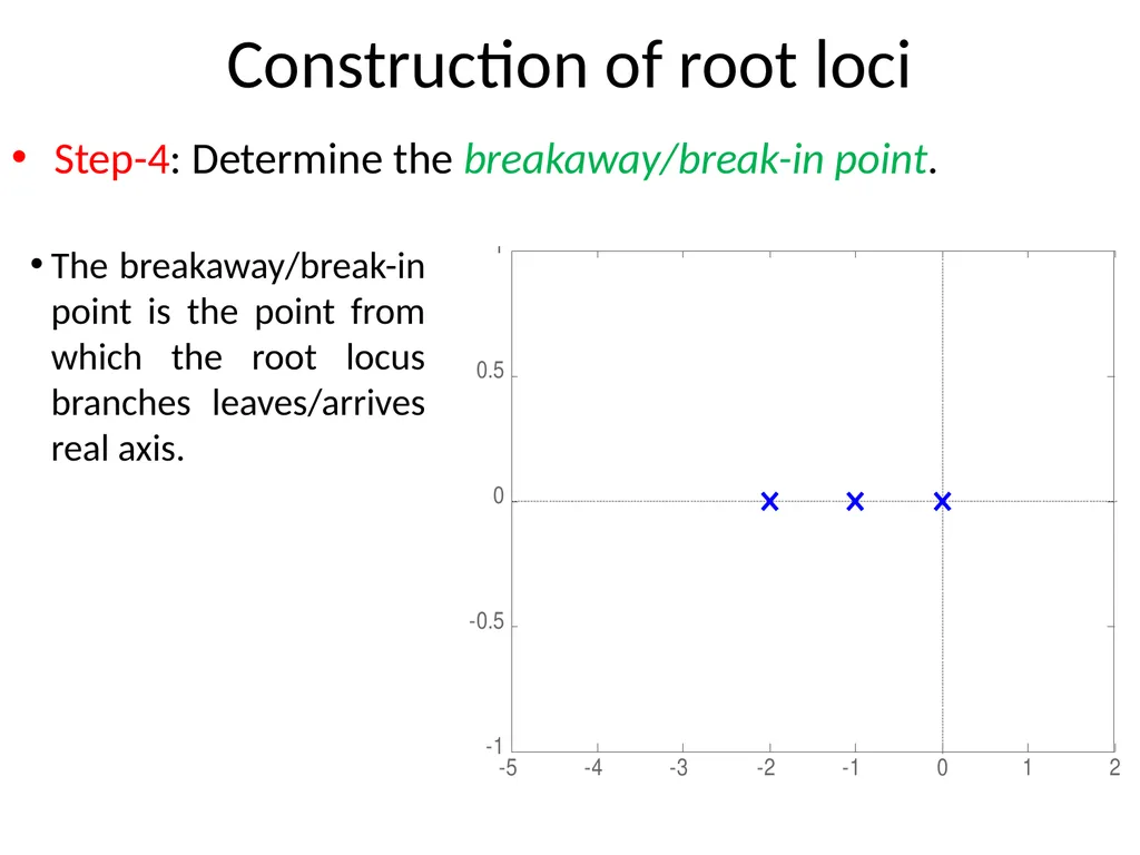
Construction of root loci Step-4: Determine the breakaway/break-in point. The breakaway/break-in point is the point from which the root locus branches leaves/arrives real axis.<br>
27
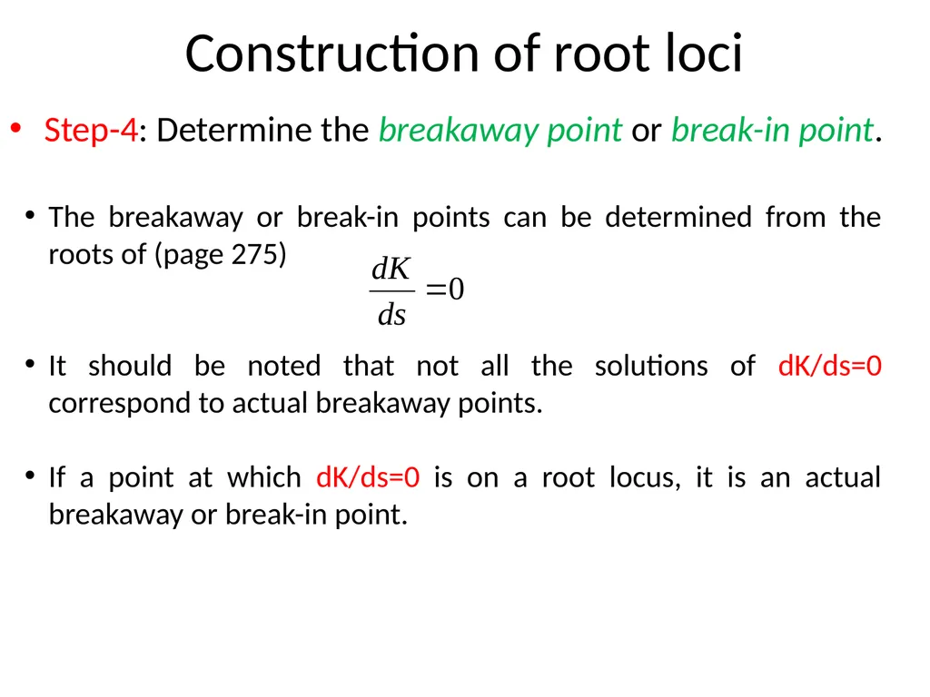
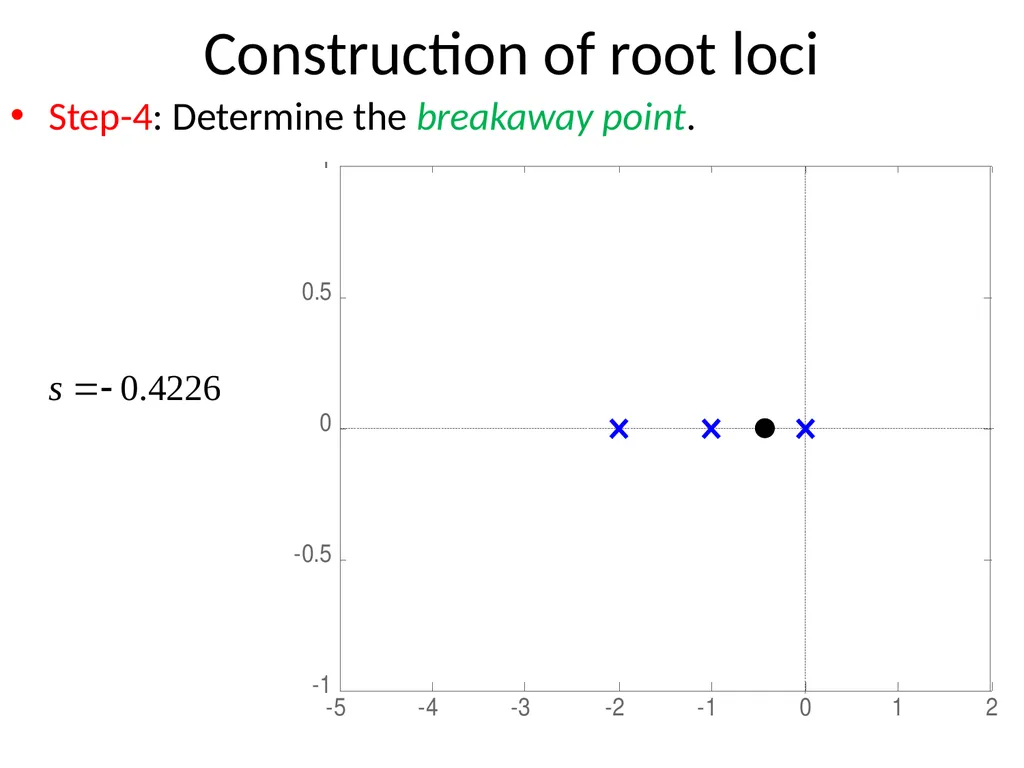
Construction of root loci Step-4: Determine the breakaway point or break-in point. The breakaway or break-in points can be determined from the roots of (page 275)
It should be noted that not all the solutions of dK/ds=0 correspond to actual breakaway points.
If a point at which dK/ds=0 is on a root locus, it is an actual breakaway or break-in point.<br>
28
Construction of root loci Step-4: Determine the breakaway point or break-in point.
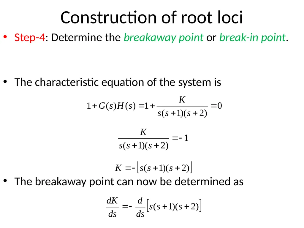
The characteristic equation of the system is
The breakaway point can now be determined as<br>
29
Construction of root loci Step-4: Determine the breakaway point or break-in point.
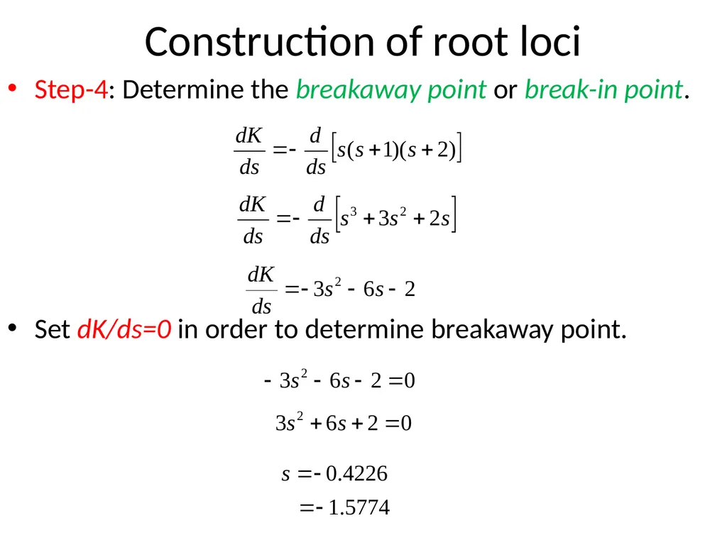
Set dK/ds=0 in order to determine breakaway point.<br>
30
Construction of root loci Step-4: Determine the breakaway point or break-in point.
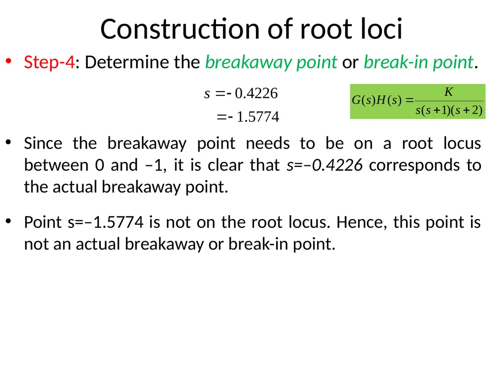
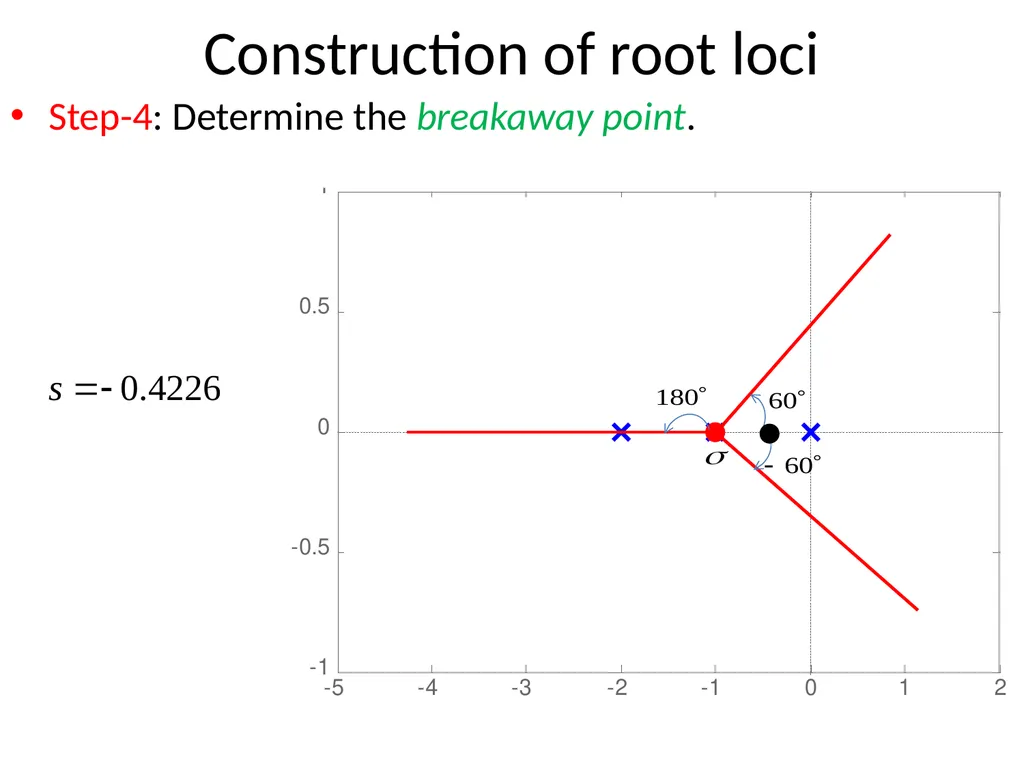
Since the breakaway point needs to be on a root locus between 0 and –1, it is clear that s=–0.4226 corresponds to the actual breakaway point.
Point s=–1.5774 is not on the root locus. Hence, this point is not an actual breakaway or break-in point.<br>
31
Construction of root loci Step-4: Determine the breakaway point.<br>
32
Construction of root loci Step-4: Determine the breakaway point.<br>
33
Construction of root loci Step-5: Determine the points where root loci cross the imaginary axis.<br>
34
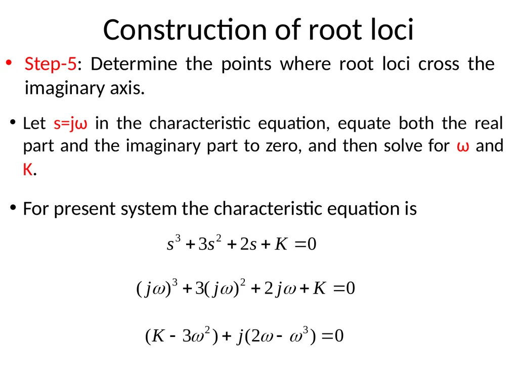
Construction of root loci Step-5: Determine the points where root loci cross the imaginary axis. Let s=jω in the characteristic equation, equate both the real part and the imaginary part to zero, and then solve for ω and K.
For present system the characteristic equation is<br>
35
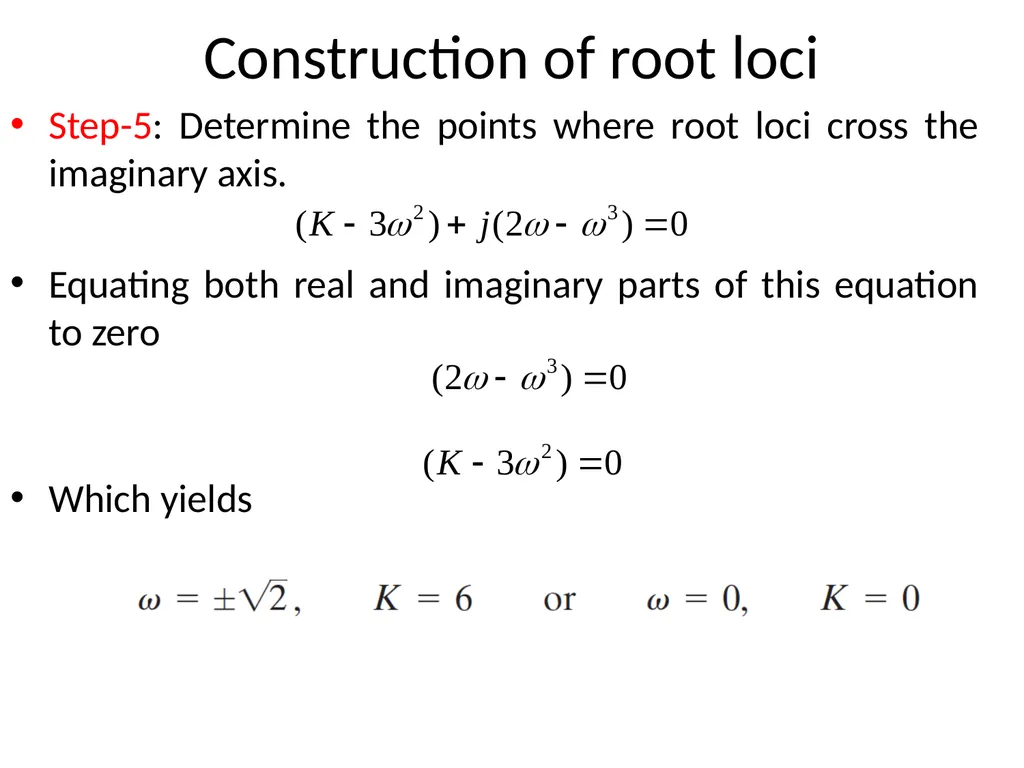
Construction of root loci Step-5: Determine the points where root loci cross the imaginary axis.
Equating both real and imaginary parts of this equation to zero
Which yields<br>
36
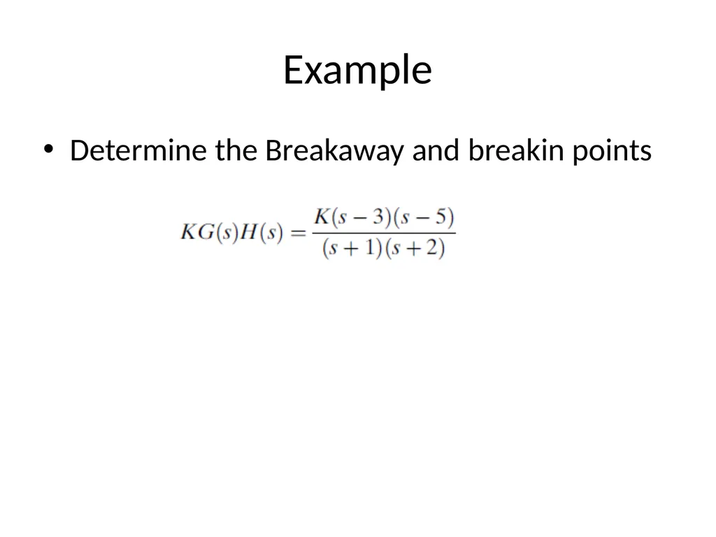
Example Determine the Breakaway and breakin points<br>
37
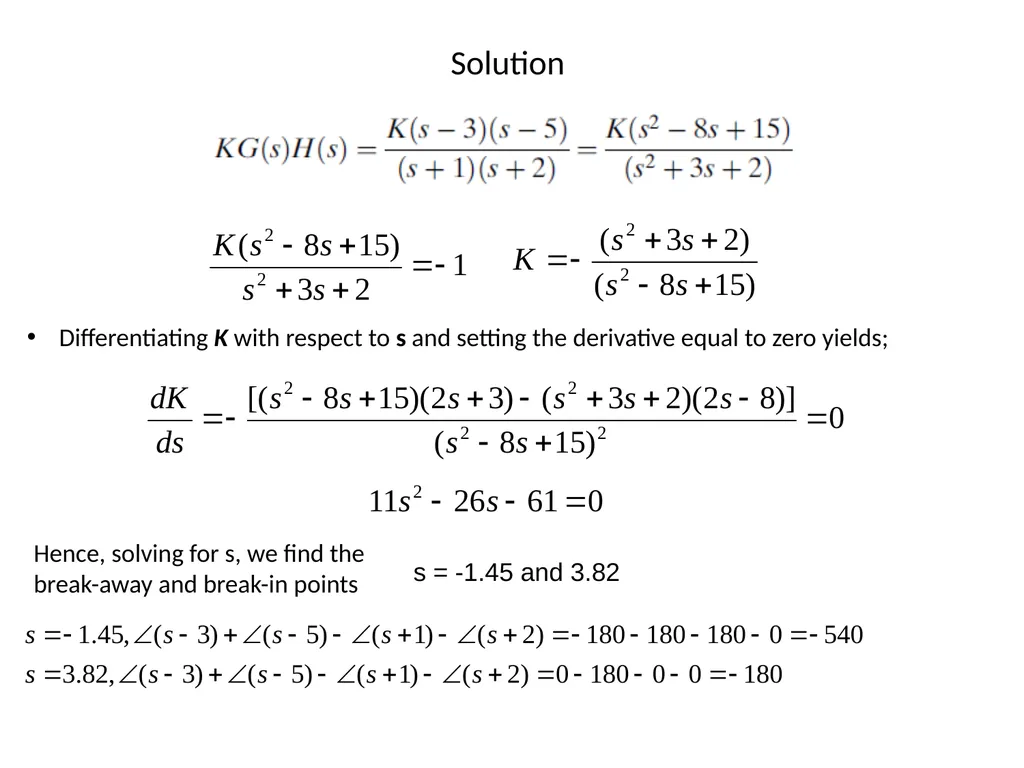
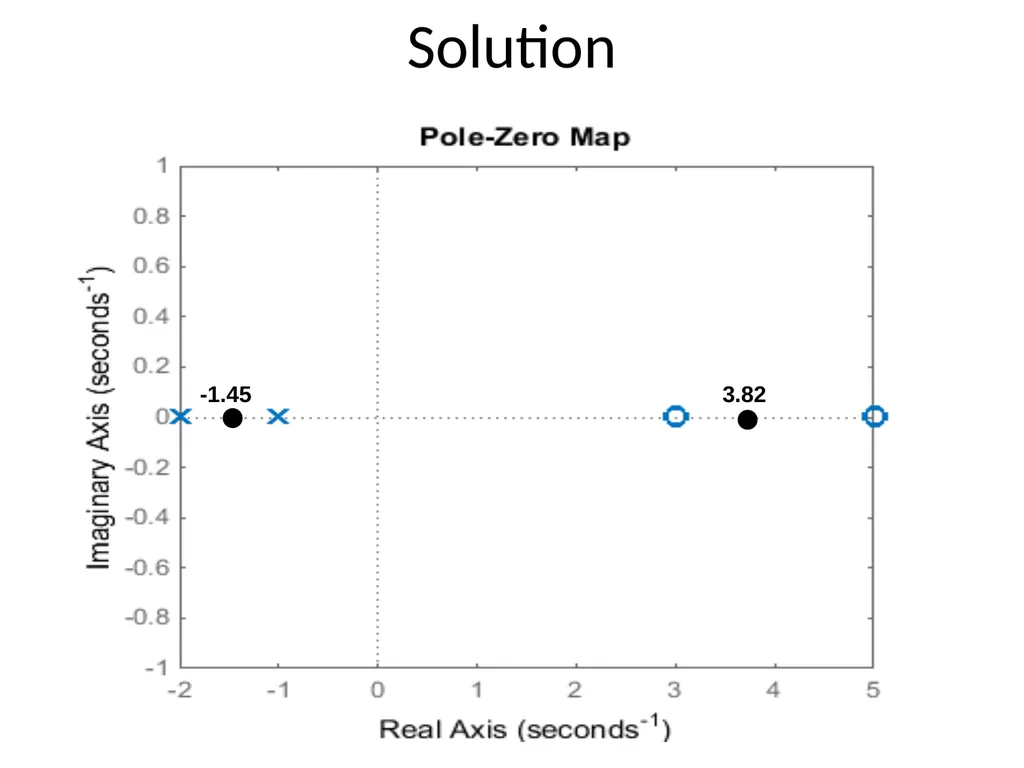
Solution Differentiating K with respect to s and setting the derivative equal to zero yields; Hence, solving for s, we find the
break-away and break-in points s = -1.45 and 3.82<br>
39
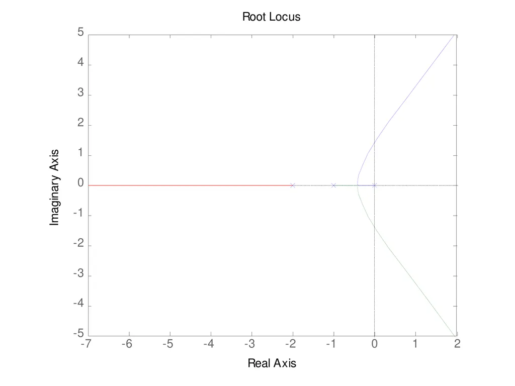
Root Loci by MATLAB Example 6-4 in page 293<br>