
Exergy, Economic Growth and Degrowth Presentation




Description: Exergy, Economic Growth and Degrowth Presentation at the International Energy Economics Workshop University of Sussex Brighton, U.K. July 13-15, 2016 Origins of Exergy-Economics Physics and thermodynamics Economic ideas since the
Related Topics
Download Presentation
"Exergy, Economic Growth and Degrowth Presentation" is the property of its rightful owner. Permission is granted to download and print the materials on this website for personal, non-commercial use only, and to display it on your personal computer provided you do not modify the materials and that you retain all copyright notices contained in the materials. By downloading content from our website, you accept the terms of this agreement.
Presentation Transcript
slide1. Exergy, Economic Growth and Degrowth Presentation at the International Energy Economics Workshop
University of Sussex
Brighton, U.K.
July 13-15, 2016<br>
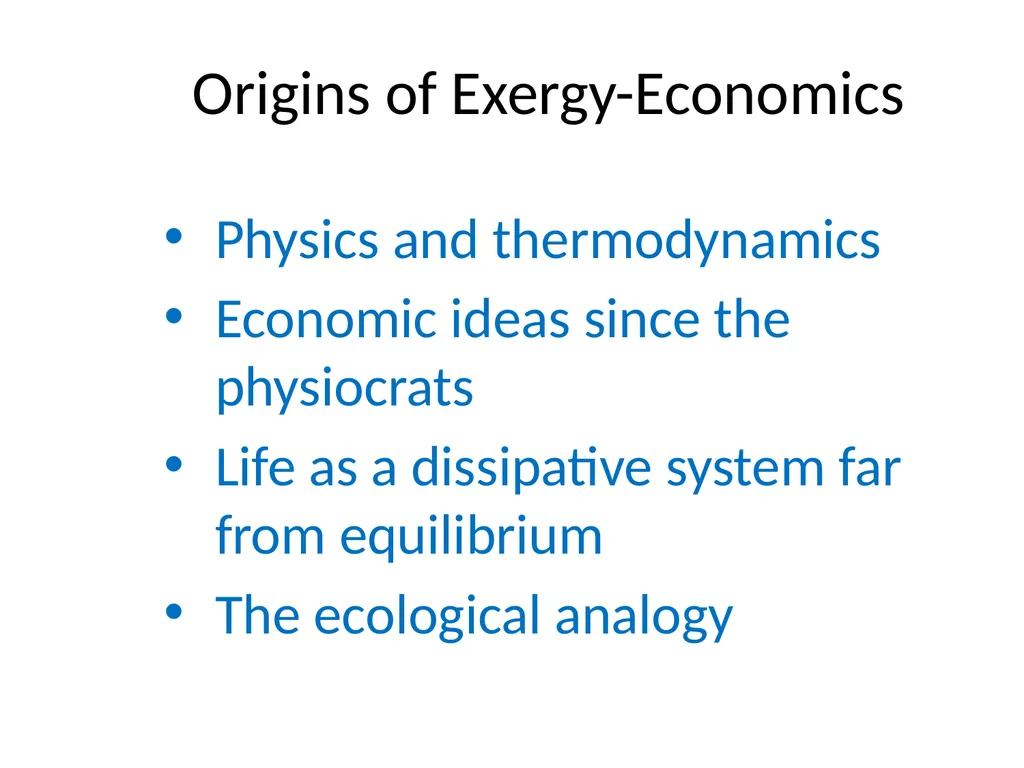
slide2. Origins of Exergy-Economics Physics and thermodynamics
Economic ideas since the physiocrats
Life as a dissipative system far from equilibrium
The ecological analogy<br>
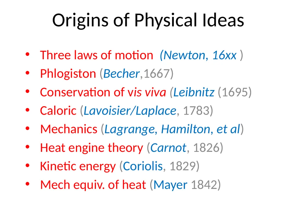
slide3. Origins of Physical Ideas Three laws of motion (Newton, 16xx )
Phlogiston (Becher,1667)
Conservation of vis viva (Leibnitz (1695)
Caloric (Lavoisier/Laplace, 1783)
Mechanics (Lagrange, Hamilton, et al)
Heat engine theory (Carnot, 1826)
Kinetic energy (Coriolis, 1829)
Mech equiv. of heat (Mayer 1842)<br>
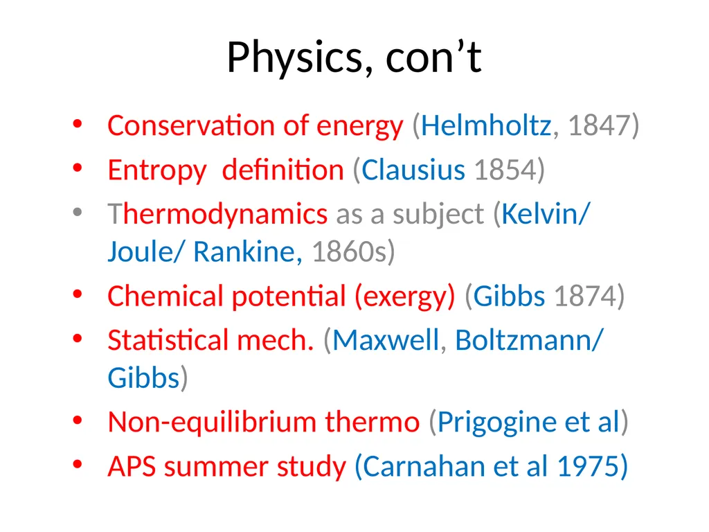
slide4. Physics, con’t Conservation of energy (Helmholtz, 1847)
Entropy definition (Clausius 1854)
Thermodynamics as a subject (Kelvin/ Joule/ Rankine, 1860s)
Chemical potential (exergy) (Gibbs 1874)
Statistical mech. (Maxwell, Boltzmann/ Gibbs)
Non-equilibrium thermo (Prigogine et al)
APS summer study (Carnahan et al 1975)<br>
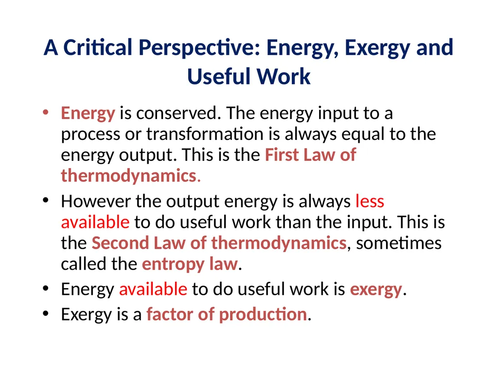
slide5. A Critical Perspective: Energy, Exergy and Useful Work Energy is conserved. The energy input to a process or transformation is always equal to the energy output. This is the First Law of thermodynamics.
However the output energy is always less available to do useful work than the input. This is the Second Law of thermodynamics, sometimes called the entropy law.
Energy available to do useful work is exergy.
Exergy is a factor of production.<br>
slide6. Exergy and Useful Work, Con’t Capital is inert. It must be activated. Most economists regard labor as the activating agent. Labor (by humans and/or animals) was once the only source of useful work in the economy.
But machines (and computers) require a different activating agent, exergy that can be converted to useful work (in the thermodynamic sense).
For economic growth models, useful work can be considered as a factor of production.<br>
slide7. Efficiency: Two kinds Energy efficiency (First Law) is “useful output” divided by total input (of energy as fuel or feedstock). This measure is quite deceptive, but common. (See slides following)
Exergy efficiency (Second Law) is a different ratio. The numerator is work actually done in the process. The denominator is the potential work (exergy) that could have been done in an ideal process allowing only for irreversibilities.<br>
slide8. Energetics, biology, ecology Energetics (Helm, 1887)
As Monism W. Ostwald (1895-…)
Technocracy H. Scott with M. King Hubbert (1931- 55)
Mathematical biology (Lotka, Rashevsky)
In ecology (H. Odum, R. Costanza, Hall, et al)
In economics & ecology (B. Hannon et al)<br>
slide9. Economics w/o Energy Trade and division of labor as source of added value (Smith, Ricardo, et al)
Labor surplus as source of wealth (Marx)
Production function of K,L (Cobb, Douglas)
Optimal growth (Ramsey, 1929)
Neoclassical growth in equilibrium (Solow, et al, 1954)
“Limits to growth” debunked (Solow, Stiglitz, Nordhaus et al, 1974…)
Endogenous theory (Romer, Lucas et al)<br>
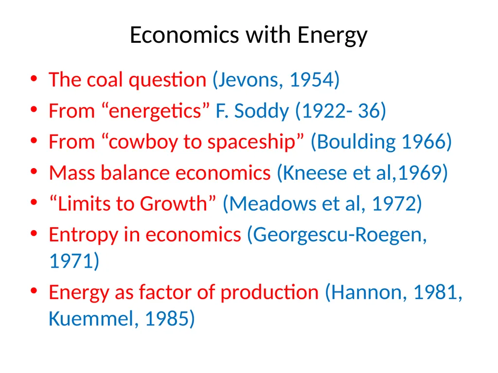
slide10. Economics with Energy The coal question (Jevons, 1954)
From “energetics” F. Soddy (1922- 36)
From “cowboy to spaceship” (Boulding 1966)
Mass balance economics (Kneese et al,1969)
“Limits to Growth” (Meadows et al, 1972)
Entropy in economics (Georgescu-Roegen, 1971)
Energy as factor of production (Hannon, 1981, Kuemmel, 1985)<br>
slide11. Most economist’s assumption #1 That resource (i.e. energy, or exergy) scarcity is not a problem. Increased consumption, from (assumed) economic growth, can be met by increased supply at no increase in price. (This was explicit in the 2010 IMF forecast and all IEA and EIA forecasts up to 2006.) It implies that the energy return on energy investments (EROEI) will be constant over time.<br>
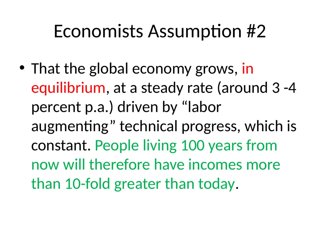
slide12. Economists Assumption #2 That the global economy grows, in equilibrium, at a steady rate (around 3 -4 percent p.a.) driven by “labor augmenting” technical progress, which is constant. People living 100 years from now will therefore have incomes more than 10-fold greater than today.<br>
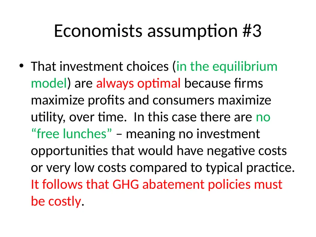
slide13. Economists assumption #3 That investment choices (in the equilibrium model) are always optimal because firms maximize profits and consumers maximize utility, over time. In this case there are no “free lunches” – meaning no investment opportunities that would have negative costs or very low costs compared to typical practice. It follows that GHG abatement policies must be costly.<br>
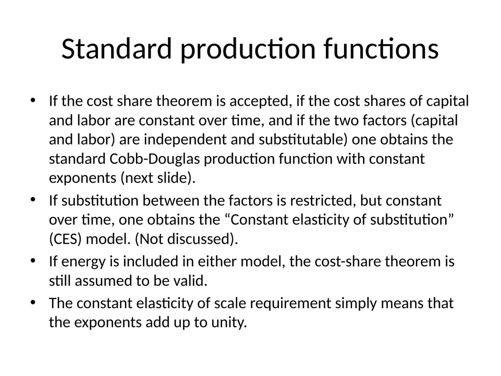
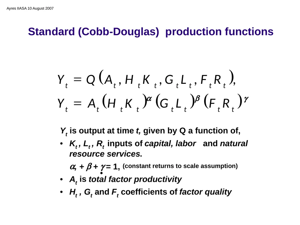
slide14. Standard production functions If the cost share theorem is accepted, if the cost shares of capital and labor are constant over time, and if the two factors (capital and labor) are independent and substitutable) one obtains the standard Cobb-Douglas production function with constant exponents (next slide).
If substitution between the factors is restricted, but constant over time, one obtains the “Constant elasticity of substitution” (CES) model. (Not discussed).
If energy is included in either model, the cost-share theorem is still assumed to be valid.
The constant elasticity of scale requirement simply means that the exponents add up to unity.<br>
slide15. Y t is output at time t, given by Q a function of, • K t , L t , R t inputs of capital, labor and natural resource services . • a , + b + g = 1, (constant returns to scale assumption) • A t is total factor productivity • H t , G t and F t coefficients of factor quality ( ) ( ) ( ) ( ) g b a t t t t t t t t t t t t t t t t R F L G K H A Y R F L G K H A Q Y = = , , , , Ayres IIASA 10 August 2007 Standard (Cobb-Douglas) production functions<br>
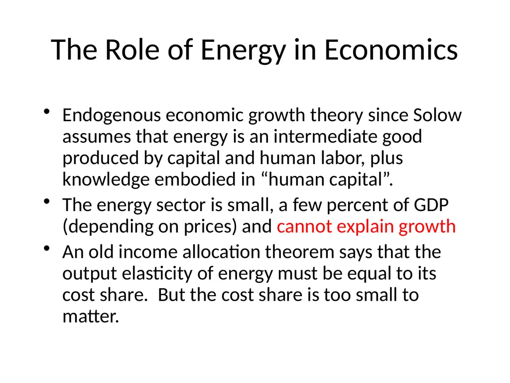
slide16. The Role of Energy in Economics Endogenous economic growth theory since Solow assumes that energy is an intermediate good produced by capital and human labor, plus knowledge embodied in “human capital”.
The energy sector is small, a few percent of GDP (depending on prices) and cannot explain growth
An old income allocation theorem says that the output elasticity of energy must be equal to its cost share. But the cost share is too small to matter.<br>
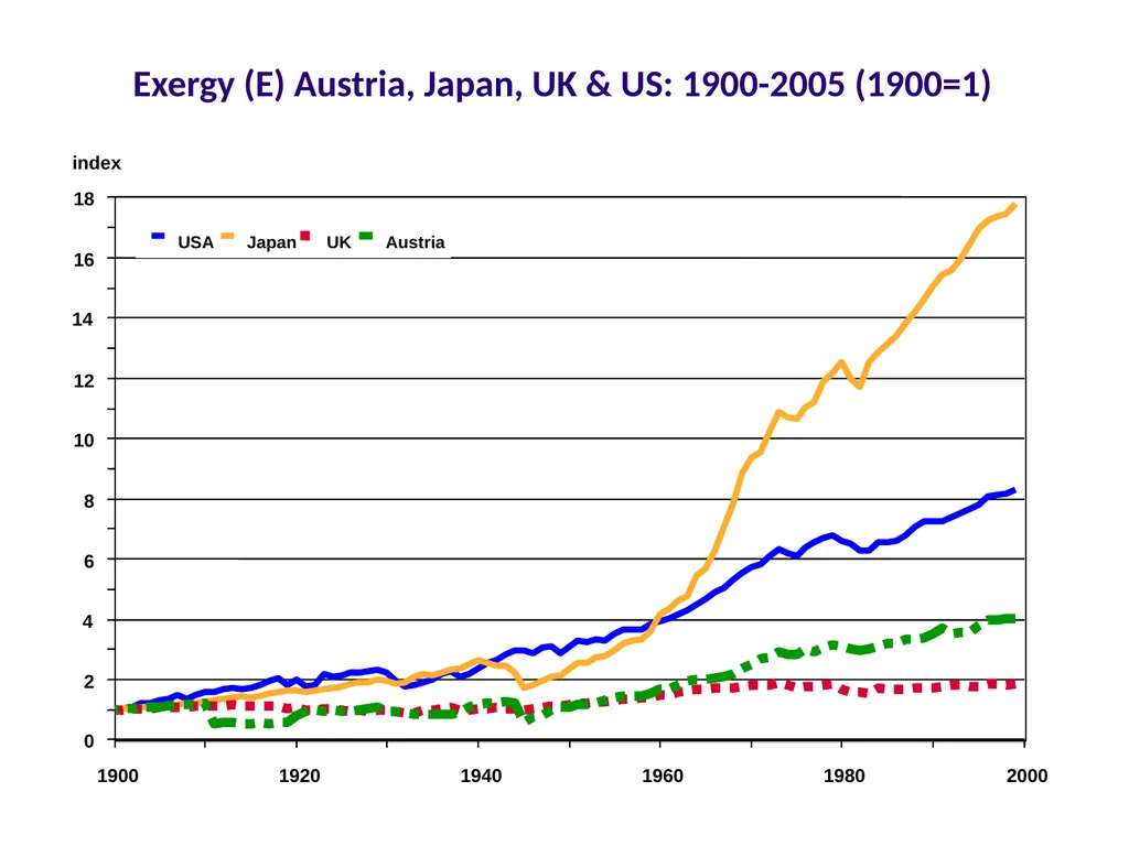
slide17. 1900 1920 1940 1960 1980 2000 0 2 4 6 8 10 12 14 16 18 index USA Japan UK Austria Exergy (E) Austria, Japan, UK & US: 1900-2005 (1900=1)<br>
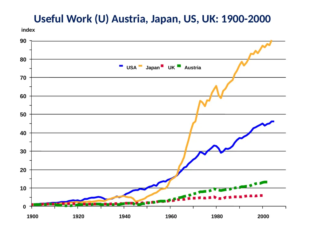
slide18. 1900 1920 1940 1960 1980 2000 0 index 10 20 30 40 50 60 70 80 90 USA Japan UK Austria Useful Work (U) Austria, Japan, US, UK: 1900-2000<br>
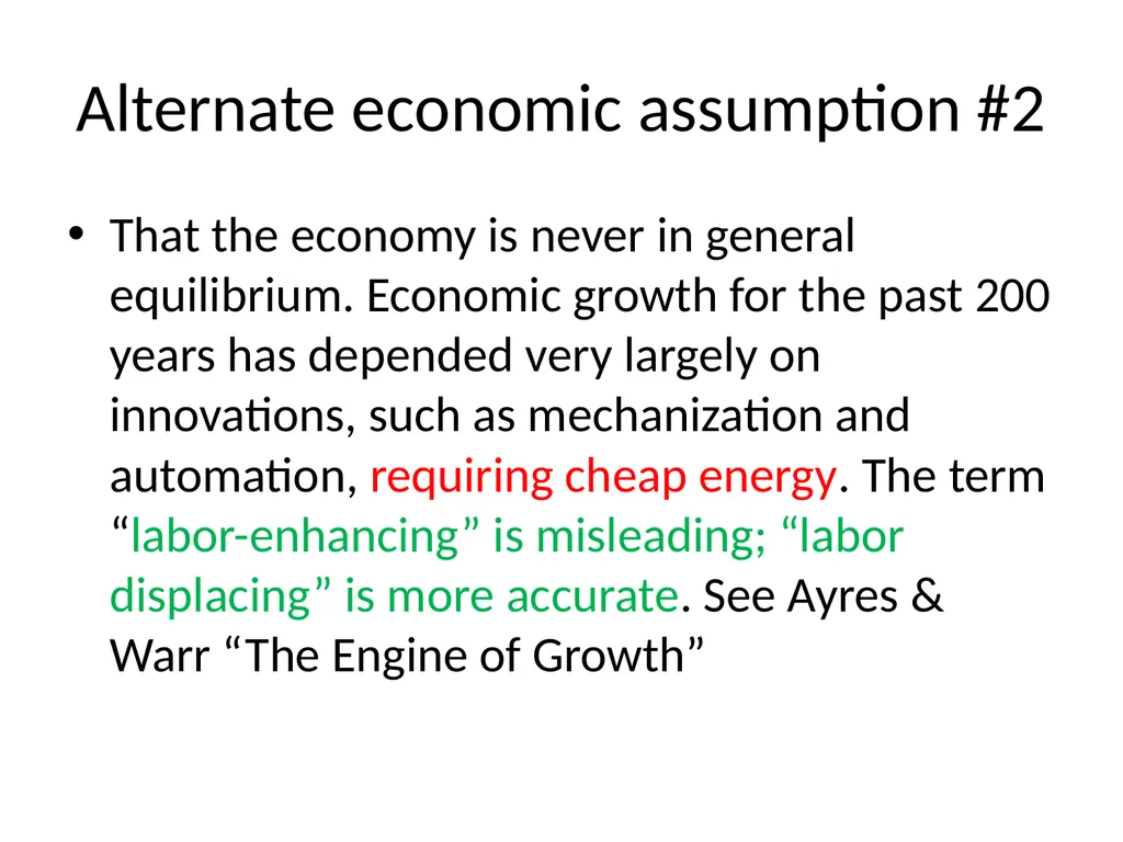
slide24. Alternate economic assumption #2 That the economy is never in general equilibrium. Economic growth for the past 200 years has depended very largely on innovations, such as mechanization and automation, requiring cheap energy. The term “labor-enhancing” is misleading; “labor displacing” is more accurate. See Ayres & Warr “The Engine of Growth”<br>
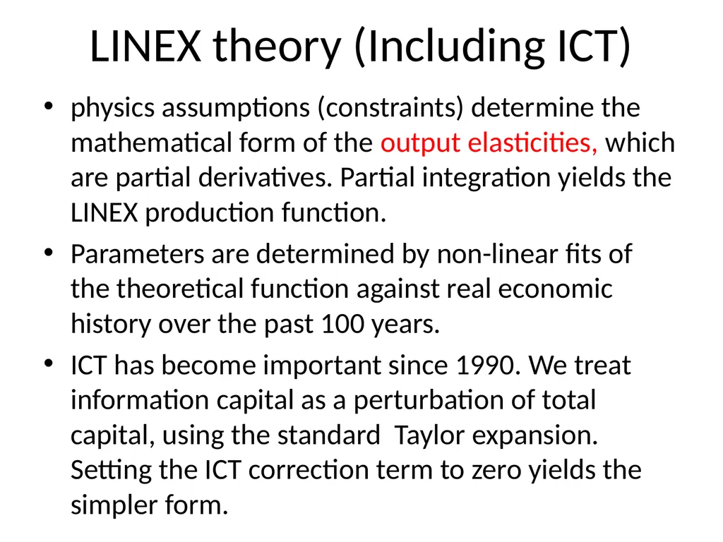
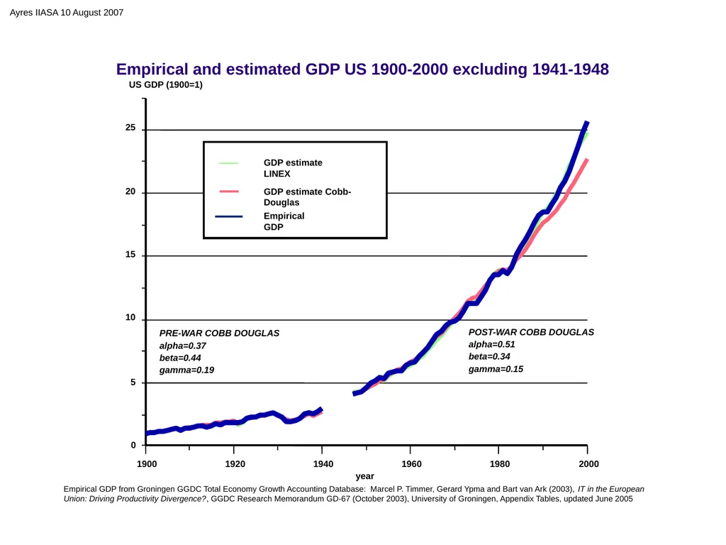
slide25. LINEX theory (Including ICT) physics assumptions (constraints) determine the mathematical form of the output elasticities, which are partial derivatives. Partial integration yields the LINEX production function.
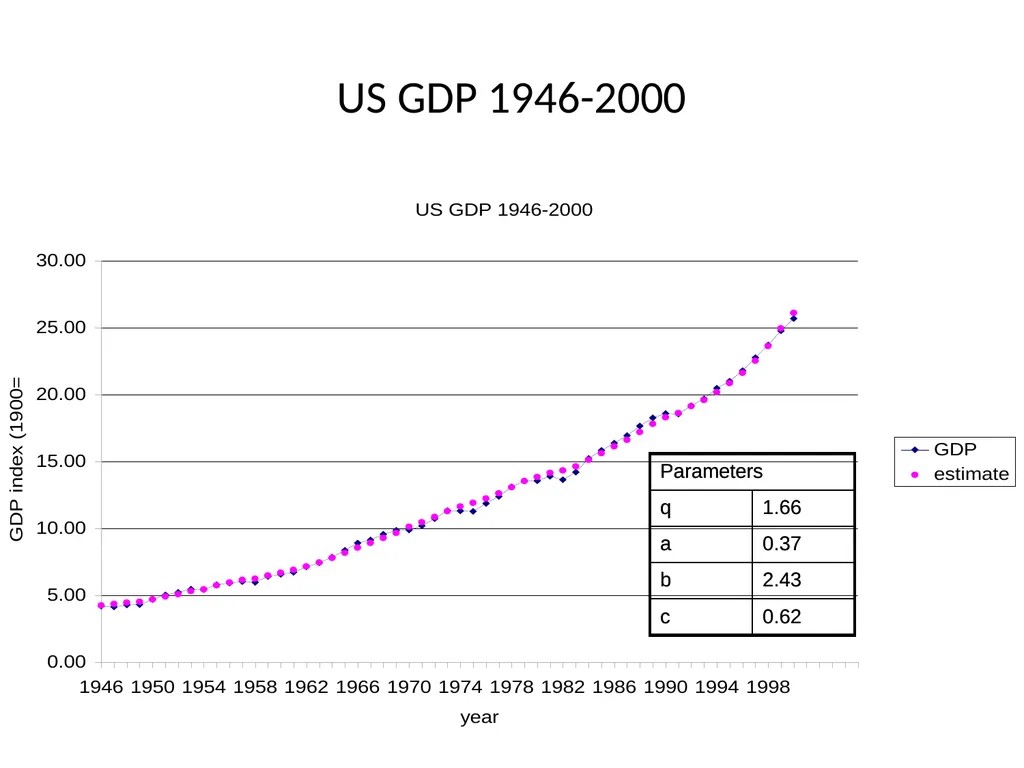
Parameters are determined by non-linear fits of the theoretical function against real economic history over the past 100 years.
ICT has become important since 1990. We treat information capital as a perturbation of total capital, using the standard Taylor expansion. Setting the ICT correction term to zero yields the simpler form.<br>
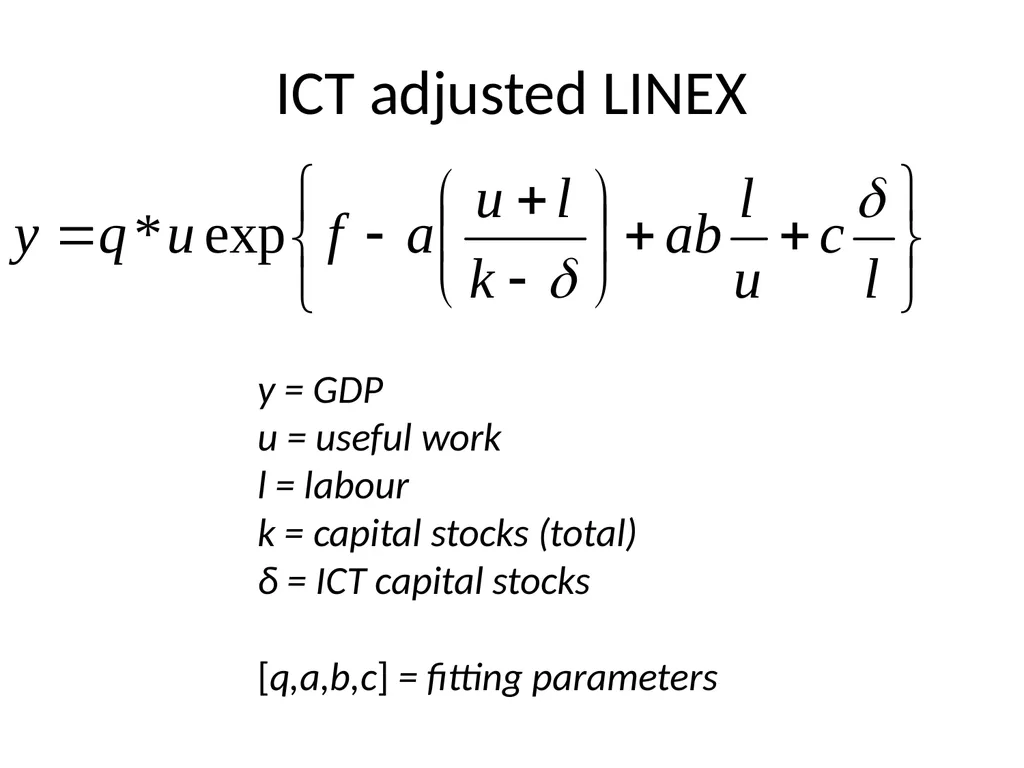
slide26. ICT adjusted LINEX y = GDP
u = useful work
l = labour
k = capital stocks (total)
δ = ICT capital stocks
[q,a,b,c] = fitting parameters<br>
slide27. 1900 1920 1940 1960 1980 2000 year 0 5 10 15 20 25 PRE-WAR COBB DOUGLAS
alpha=0.37
beta=0.44
gamma=0.19 POST-WAR COBB DOUGLAS
alpha=0.51
beta=0.34
gamma=0.15 GDP estimate LINEX GDP estimate Cobb-Douglas Empirical GDP US GDP (1900=1) Empirical GDP from Groningen GGDC Total Economy Growth Accounting Database: Marcel P. Timmer, Gerard Ypma and Bart van Ark (2003), IT in the European Union: Driving Productivity Divergence?, GGDC Research Memorandum GD-67 (October 2003), University of Groningen, Appendix Tables, updated June 2005 Ayres IIASA 10 August 2007 Empirical and estimated GDP US 1900-2000 excluding 1941-1948<br>
slide28. US GDP 1946-2000<br>
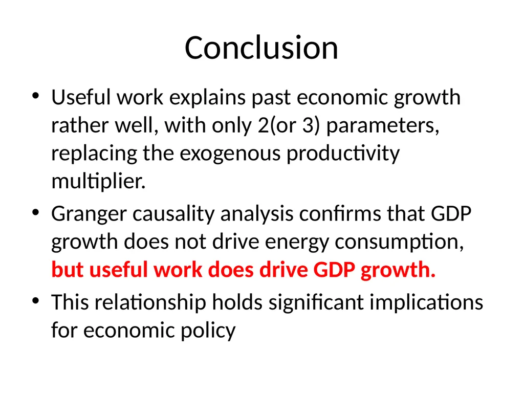
slide29. Conclusion Useful work explains past economic growth rather well, with only 2(or 3) parameters, replacing the exogenous productivity multiplier.
Granger causality analysis confirms that GDP growth does not drive energy consumption, but useful work does drive GDP growth.
This relationship holds significant implications for economic policy<br>
slide30. I’ll stop here. Thanks for listening The rest is an Appendix<br>
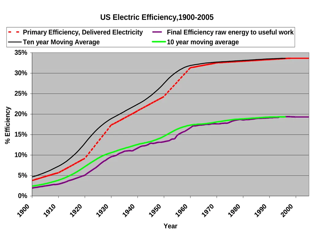
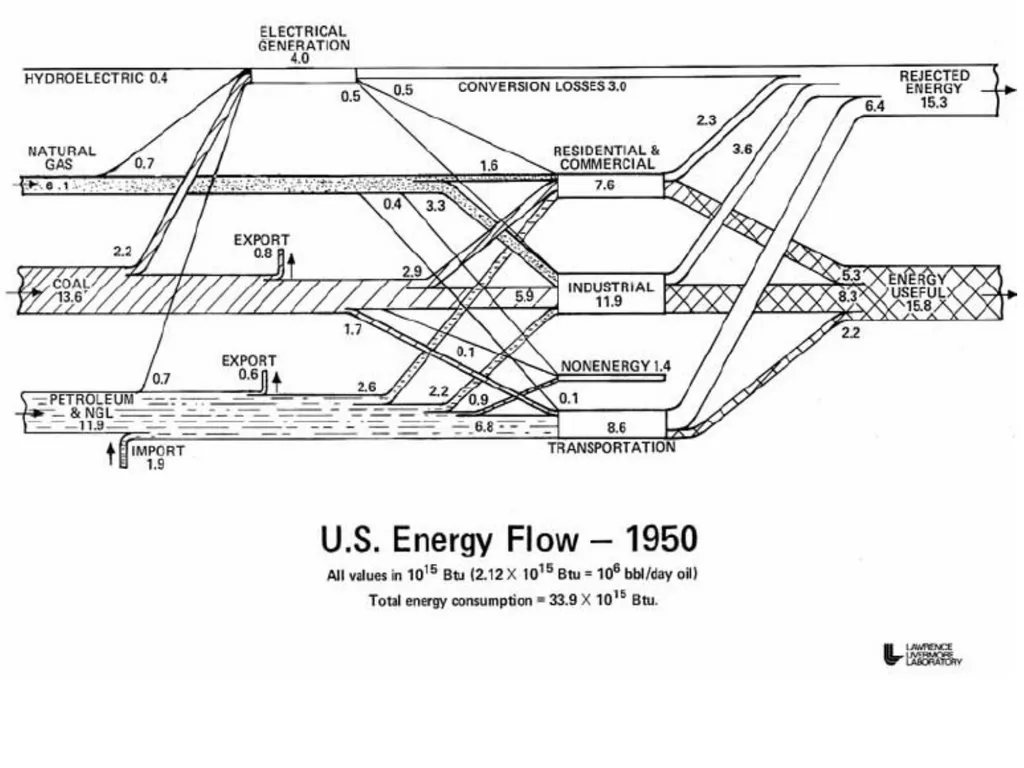
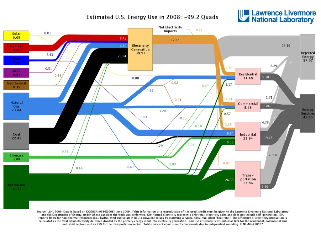
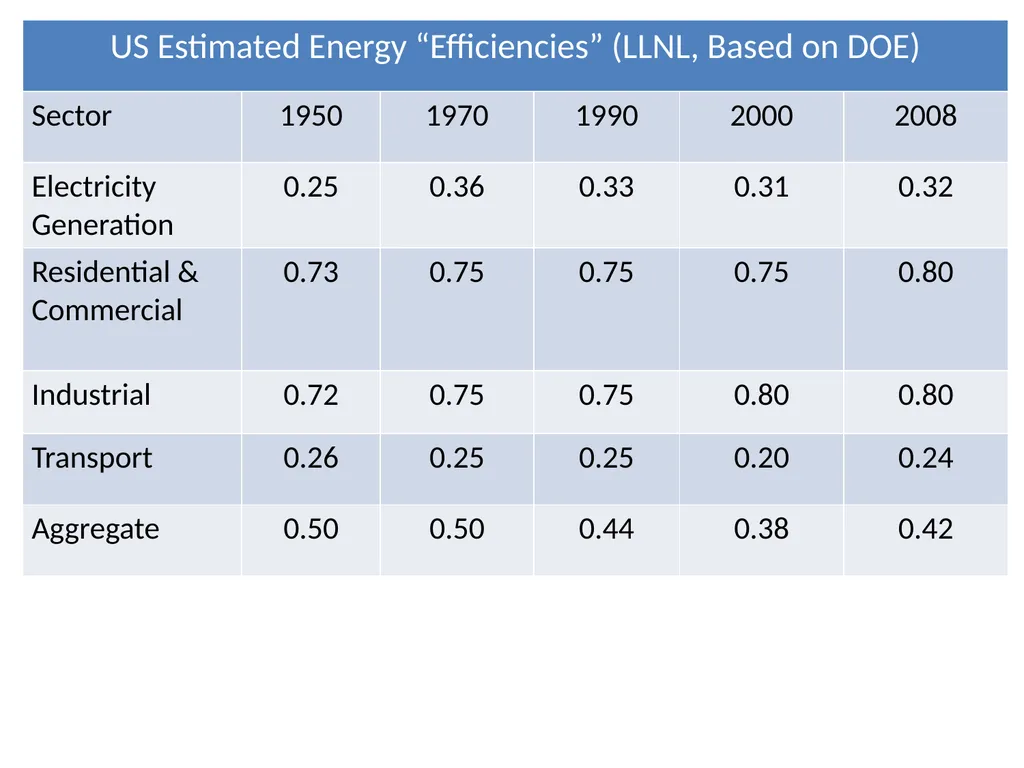
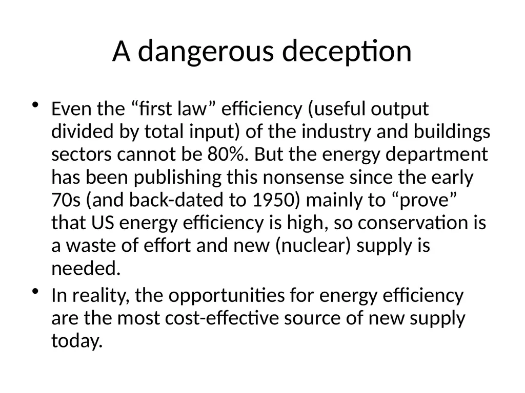
slide34. A dangerous deception Even the “first law” efficiency (useful output divided by total input) of the industry and buildings sectors cannot be 80%. But the energy department has been publishing this nonsense since the early 70s (and back-dated to 1950) mainly to “prove” that US energy efficiency is high, so conservation is a waste of effort and new (nuclear) supply is needed.
In reality, the opportunities for energy efficiency are the most cost-effective source of new supply today.<br>
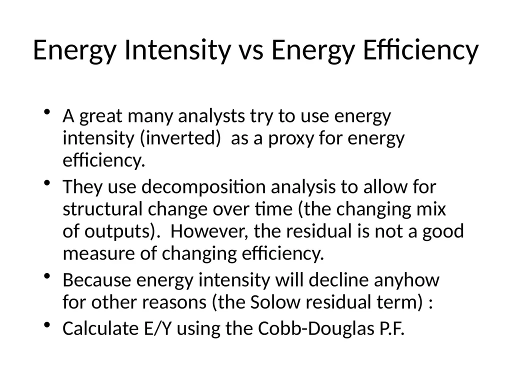
slide35. Energy Intensity vs Energy Efficiency A great many analysts try to use energy intensity (inverted) as a proxy for energy efficiency.
They use decomposition analysis to allow for structural change over time (the changing mix of outputs). However, the residual is not a good measure of changing efficiency.
Because energy intensity will decline anyhow for other reasons (the Solow residual term) :
Calculate E/Y using the Cobb-Douglas P.F.<br>
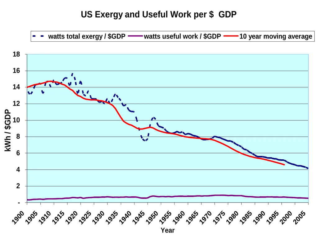
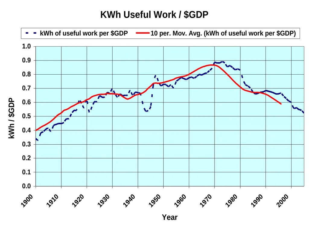
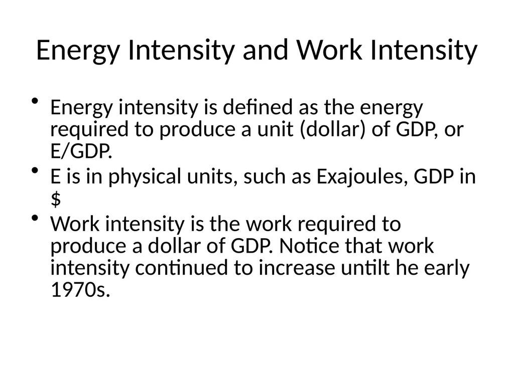
slide36. Energy Intensity and Work Intensity Energy intensity is defined as the energy required to produce a unit (dollar) of GDP, or E/GDP.
E is in physical units, such as Exajoules, GDP in $
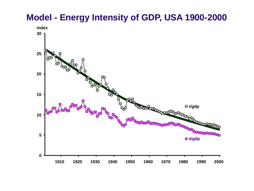
Work intensity is the work required to produce a dollar of GDP. Notice that work intensity continued to increase untilt he early 1970s.<br>
slide37. Model - Energy Intensity of GDP, USA 1900-2000 0 5 10 15 20 25 30 2000 1990 1980 1970 1960 1950 1940 1930 1920 1910 index r/gdp e/gdp<br>
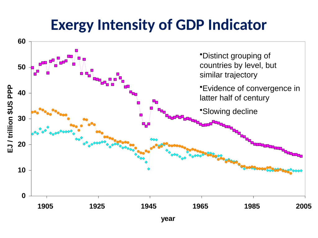
slide38. Exergy Intensity of GDP Indicator Distinct grouping of countries by level, but similar trajectory
Evidence of convergence in latter half of century
Slowing decline<br>
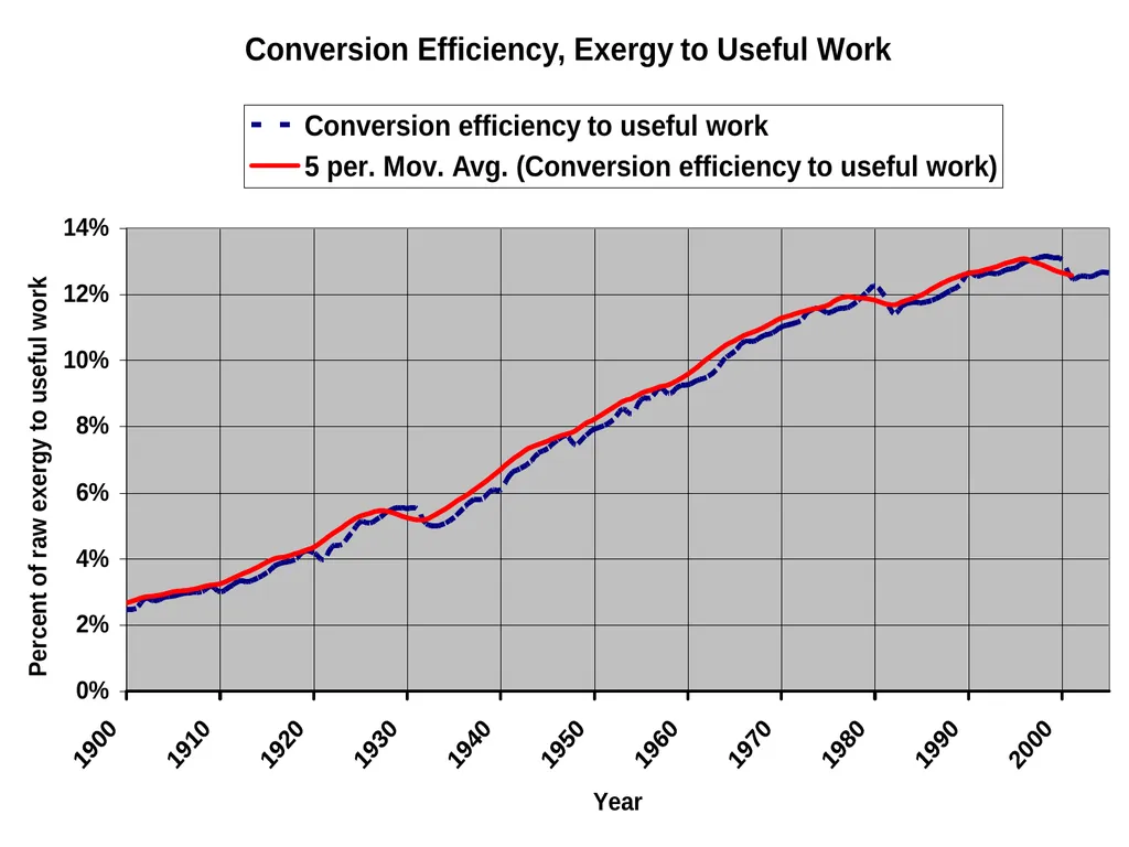
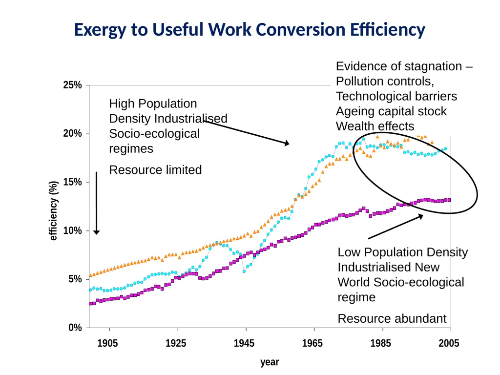
slide39. Exergy to Useful Work Conversion Efficiency<br>
University of Sussex
Brighton, U.K.
July 13-15, 2016<br>
slide2. Origins of Exergy-Economics Physics and thermodynamics
Economic ideas since the physiocrats
Life as a dissipative system far from equilibrium
The ecological analogy<br>
slide3. Origins of Physical Ideas Three laws of motion (Newton, 16xx )
Phlogiston (Becher,1667)
Conservation of vis viva (Leibnitz (1695)
Caloric (Lavoisier/Laplace, 1783)
Mechanics (Lagrange, Hamilton, et al)
Heat engine theory (Carnot, 1826)
Kinetic energy (Coriolis, 1829)
Mech equiv. of heat (Mayer 1842)<br>
slide4. Physics, con’t Conservation of energy (Helmholtz, 1847)
Entropy definition (Clausius 1854)
Thermodynamics as a subject (Kelvin/ Joule/ Rankine, 1860s)
Chemical potential (exergy) (Gibbs 1874)
Statistical mech. (Maxwell, Boltzmann/ Gibbs)
Non-equilibrium thermo (Prigogine et al)
APS summer study (Carnahan et al 1975)<br>
slide5. A Critical Perspective: Energy, Exergy and Useful Work Energy is conserved. The energy input to a process or transformation is always equal to the energy output. This is the First Law of thermodynamics.
However the output energy is always less available to do useful work than the input. This is the Second Law of thermodynamics, sometimes called the entropy law.
Energy available to do useful work is exergy.
Exergy is a factor of production.<br>
slide6. Exergy and Useful Work, Con’t Capital is inert. It must be activated. Most economists regard labor as the activating agent. Labor (by humans and/or animals) was once the only source of useful work in the economy.
But machines (and computers) require a different activating agent, exergy that can be converted to useful work (in the thermodynamic sense).
For economic growth models, useful work can be considered as a factor of production.<br>
slide7. Efficiency: Two kinds Energy efficiency (First Law) is “useful output” divided by total input (of energy as fuel or feedstock). This measure is quite deceptive, but common. (See slides following)
Exergy efficiency (Second Law) is a different ratio. The numerator is work actually done in the process. The denominator is the potential work (exergy) that could have been done in an ideal process allowing only for irreversibilities.<br>
slide8. Energetics, biology, ecology Energetics (Helm, 1887)
As Monism W. Ostwald (1895-…)
Technocracy H. Scott with M. King Hubbert (1931- 55)
Mathematical biology (Lotka, Rashevsky)
In ecology (H. Odum, R. Costanza, Hall, et al)
In economics & ecology (B. Hannon et al)<br>
slide9. Economics w/o Energy Trade and division of labor as source of added value (Smith, Ricardo, et al)
Labor surplus as source of wealth (Marx)
Production function of K,L (Cobb, Douglas)
Optimal growth (Ramsey, 1929)
Neoclassical growth in equilibrium (Solow, et al, 1954)
“Limits to growth” debunked (Solow, Stiglitz, Nordhaus et al, 1974…)
Endogenous theory (Romer, Lucas et al)<br>
slide10. Economics with Energy The coal question (Jevons, 1954)
From “energetics” F. Soddy (1922- 36)
From “cowboy to spaceship” (Boulding 1966)
Mass balance economics (Kneese et al,1969)
“Limits to Growth” (Meadows et al, 1972)
Entropy in economics (Georgescu-Roegen, 1971)
Energy as factor of production (Hannon, 1981, Kuemmel, 1985)<br>
slide11. Most economist’s assumption #1 That resource (i.e. energy, or exergy) scarcity is not a problem. Increased consumption, from (assumed) economic growth, can be met by increased supply at no increase in price. (This was explicit in the 2010 IMF forecast and all IEA and EIA forecasts up to 2006.) It implies that the energy return on energy investments (EROEI) will be constant over time.<br>
slide12. Economists Assumption #2 That the global economy grows, in equilibrium, at a steady rate (around 3 -4 percent p.a.) driven by “labor augmenting” technical progress, which is constant. People living 100 years from now will therefore have incomes more than 10-fold greater than today.<br>
slide13. Economists assumption #3 That investment choices (in the equilibrium model) are always optimal because firms maximize profits and consumers maximize utility, over time. In this case there are no “free lunches” – meaning no investment opportunities that would have negative costs or very low costs compared to typical practice. It follows that GHG abatement policies must be costly.<br>
slide14. Standard production functions If the cost share theorem is accepted, if the cost shares of capital and labor are constant over time, and if the two factors (capital and labor) are independent and substitutable) one obtains the standard Cobb-Douglas production function with constant exponents (next slide).
If substitution between the factors is restricted, but constant over time, one obtains the “Constant elasticity of substitution” (CES) model. (Not discussed).
If energy is included in either model, the cost-share theorem is still assumed to be valid.
The constant elasticity of scale requirement simply means that the exponents add up to unity.<br>
slide15. Y t is output at time t, given by Q a function of, • K t , L t , R t inputs of capital, labor and natural resource services . • a , + b + g = 1, (constant returns to scale assumption) • A t is total factor productivity • H t , G t and F t coefficients of factor quality ( ) ( ) ( ) ( ) g b a t t t t t t t t t t t t t t t t R F L G K H A Y R F L G K H A Q Y = = , , , , Ayres IIASA 10 August 2007 Standard (Cobb-Douglas) production functions<br>
slide16. The Role of Energy in Economics Endogenous economic growth theory since Solow assumes that energy is an intermediate good produced by capital and human labor, plus knowledge embodied in “human capital”.
The energy sector is small, a few percent of GDP (depending on prices) and cannot explain growth
An old income allocation theorem says that the output elasticity of energy must be equal to its cost share. But the cost share is too small to matter.<br>
slide17. 1900 1920 1940 1960 1980 2000 0 2 4 6 8 10 12 14 16 18 index USA Japan UK Austria Exergy (E) Austria, Japan, UK & US: 1900-2005 (1900=1)<br>
slide18. 1900 1920 1940 1960 1980 2000 0 index 10 20 30 40 50 60 70 80 90 USA Japan UK Austria Useful Work (U) Austria, Japan, US, UK: 1900-2000<br>
slide24. Alternate economic assumption #2 That the economy is never in general equilibrium. Economic growth for the past 200 years has depended very largely on innovations, such as mechanization and automation, requiring cheap energy. The term “labor-enhancing” is misleading; “labor displacing” is more accurate. See Ayres & Warr “The Engine of Growth”<br>
slide25. LINEX theory (Including ICT) physics assumptions (constraints) determine the mathematical form of the output elasticities, which are partial derivatives. Partial integration yields the LINEX production function.
Parameters are determined by non-linear fits of the theoretical function against real economic history over the past 100 years.
ICT has become important since 1990. We treat information capital as a perturbation of total capital, using the standard Taylor expansion. Setting the ICT correction term to zero yields the simpler form.<br>
slide26. ICT adjusted LINEX y = GDP
u = useful work
l = labour
k = capital stocks (total)
δ = ICT capital stocks
[q,a,b,c] = fitting parameters<br>
slide27. 1900 1920 1940 1960 1980 2000 year 0 5 10 15 20 25 PRE-WAR COBB DOUGLAS
alpha=0.37
beta=0.44
gamma=0.19 POST-WAR COBB DOUGLAS
alpha=0.51
beta=0.34
gamma=0.15 GDP estimate LINEX GDP estimate Cobb-Douglas Empirical GDP US GDP (1900=1) Empirical GDP from Groningen GGDC Total Economy Growth Accounting Database: Marcel P. Timmer, Gerard Ypma and Bart van Ark (2003), IT in the European Union: Driving Productivity Divergence?, GGDC Research Memorandum GD-67 (October 2003), University of Groningen, Appendix Tables, updated June 2005 Ayres IIASA 10 August 2007 Empirical and estimated GDP US 1900-2000 excluding 1941-1948<br>
slide28. US GDP 1946-2000<br>
slide29. Conclusion Useful work explains past economic growth rather well, with only 2(or 3) parameters, replacing the exogenous productivity multiplier.
Granger causality analysis confirms that GDP growth does not drive energy consumption, but useful work does drive GDP growth.
This relationship holds significant implications for economic policy<br>
slide30. I’ll stop here. Thanks for listening The rest is an Appendix<br>
slide34. A dangerous deception Even the “first law” efficiency (useful output divided by total input) of the industry and buildings sectors cannot be 80%. But the energy department has been publishing this nonsense since the early 70s (and back-dated to 1950) mainly to “prove” that US energy efficiency is high, so conservation is a waste of effort and new (nuclear) supply is needed.
In reality, the opportunities for energy efficiency are the most cost-effective source of new supply today.<br>
slide35. Energy Intensity vs Energy Efficiency A great many analysts try to use energy intensity (inverted) as a proxy for energy efficiency.
They use decomposition analysis to allow for structural change over time (the changing mix of outputs). However, the residual is not a good measure of changing efficiency.
Because energy intensity will decline anyhow for other reasons (the Solow residual term) :
Calculate E/Y using the Cobb-Douglas P.F.<br>
slide36. Energy Intensity and Work Intensity Energy intensity is defined as the energy required to produce a unit (dollar) of GDP, or E/GDP.
E is in physical units, such as Exajoules, GDP in $
Work intensity is the work required to produce a dollar of GDP. Notice that work intensity continued to increase untilt he early 1970s.<br>
slide37. Model - Energy Intensity of GDP, USA 1900-2000 0 5 10 15 20 25 30 2000 1990 1980 1970 1960 1950 1940 1930 1920 1910 index r/gdp e/gdp<br>
slide38. Exergy Intensity of GDP Indicator Distinct grouping of countries by level, but similar trajectory
Evidence of convergence in latter half of century
Slowing decline<br>
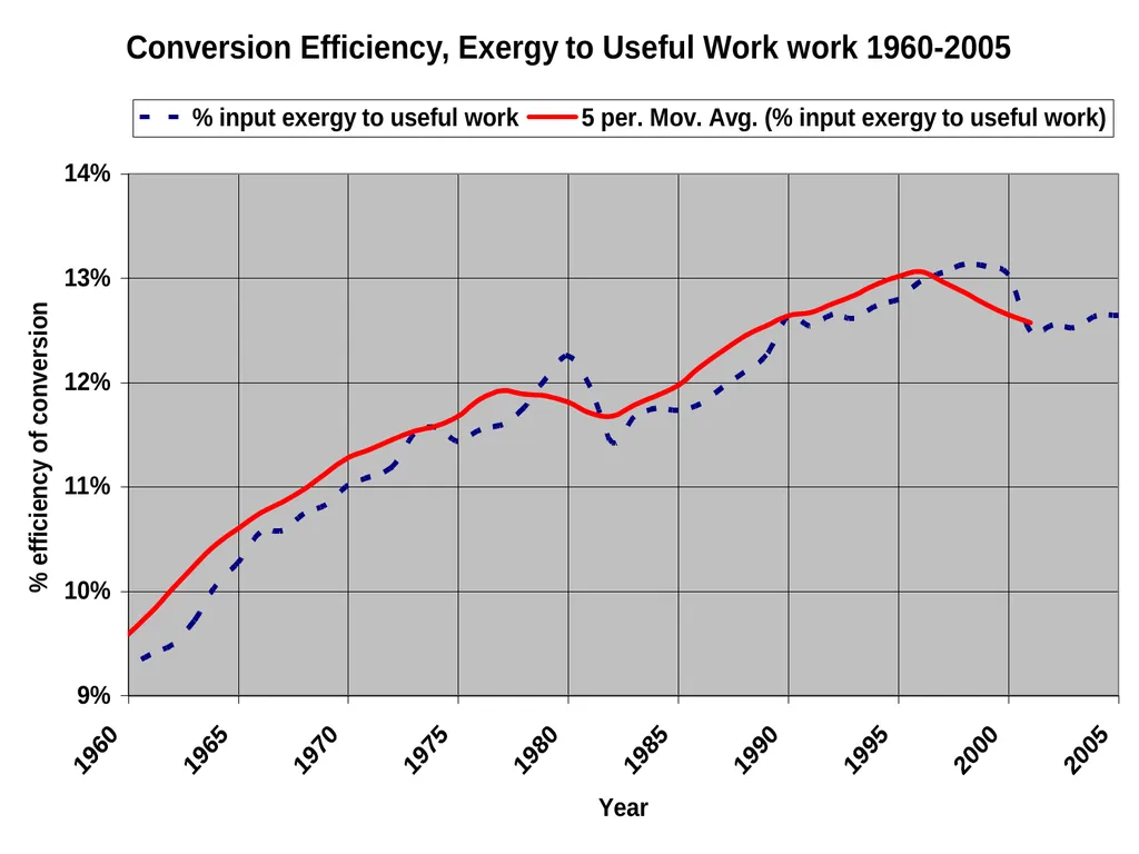
slide39. Exergy to Useful Work Conversion Efficiency<br>