02
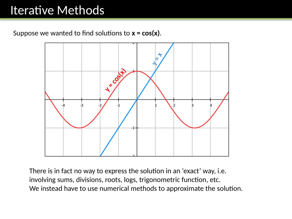
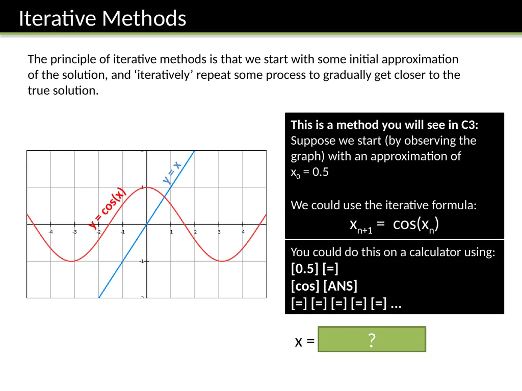
y = x y = cos(x) Suppose we wanted to find solutions to x = cos(x). There is in fact no way to express the solution in an ‘exact’ way, i.e. involving sums, divisions, roots, logs, trigonometric function, etc.
We instead have to use numerical methods to approximate the solution.<br>
04
There are different numerical methods we could use.
Why have different methods? Some converge to the solution more quickly than others. Some methods may not converge at all for certain equations/initial choice of x, either diverging, or oscillating between values. 1 2 For FP1 we will be exploring 3 root-finding algorithms:
Interval Bisection
Linear Interpolation
Newton-Rhapson Process
These will all be used to find the roots of functions, i.e. the x for which f(x) = 0.<br>
05
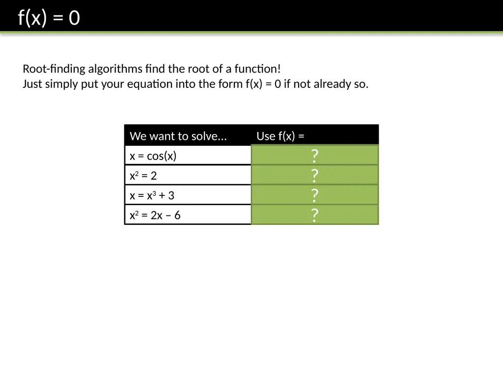
Root-finding algorithms find the root of a function!
Just simply put your equation into the form f(x) = 0 if not already so. We want to solve... x = cos(x) Use f(x) = f(x) = x – cos(x) x2 = 2 f(x) = x2 – 2 x = x3 + 3 f(x) = x3 – x + 3 x2 = 2x – 6 f(x) = x2 – 2x + 6 ? ? ? ?<br>
06
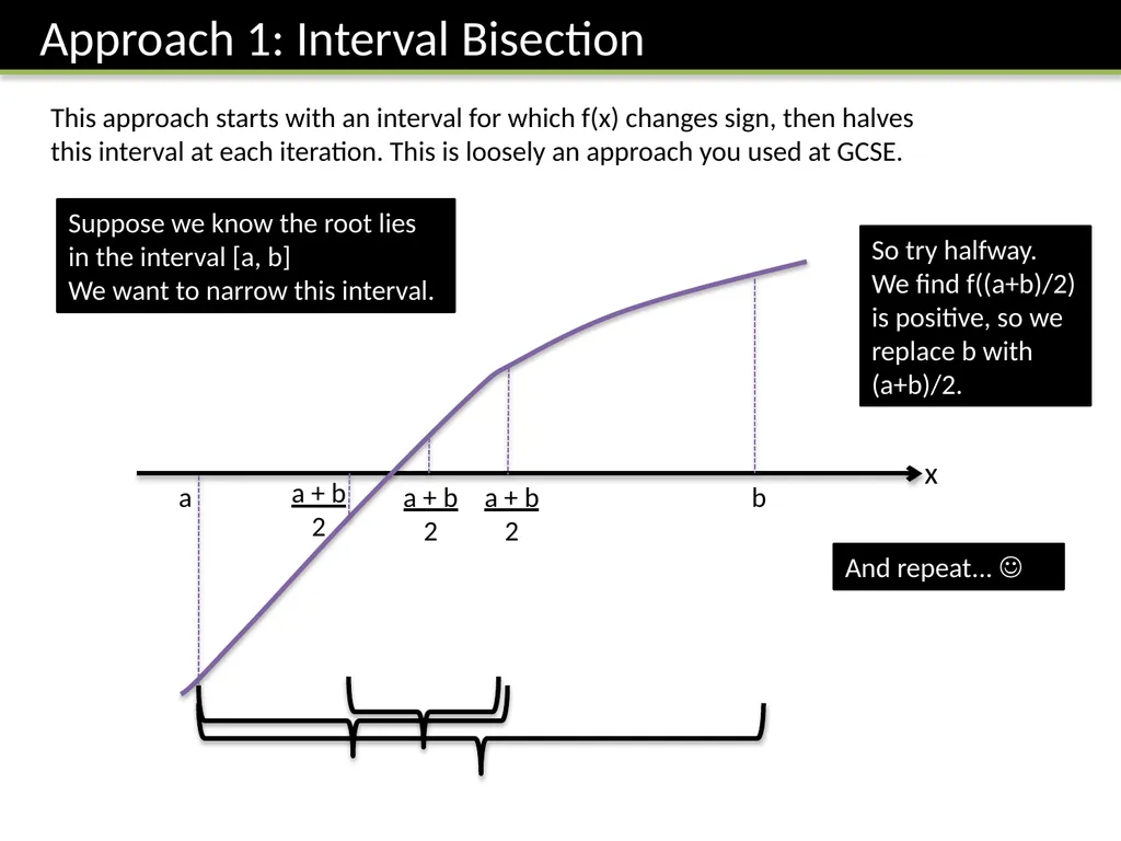
This approach starts with an interval for which f(x) changes sign, then halves this interval at each iteration. This is loosely an approach you used at GCSE. x a b Suppose we know the root lies in the interval [a, b]
We want to narrow this interval. a + b
2 So try halfway. We find f((a+b)/2) is positive, so we replace b with (a+b)/2. And repeat... a + b
2 a + b
2<br>
07
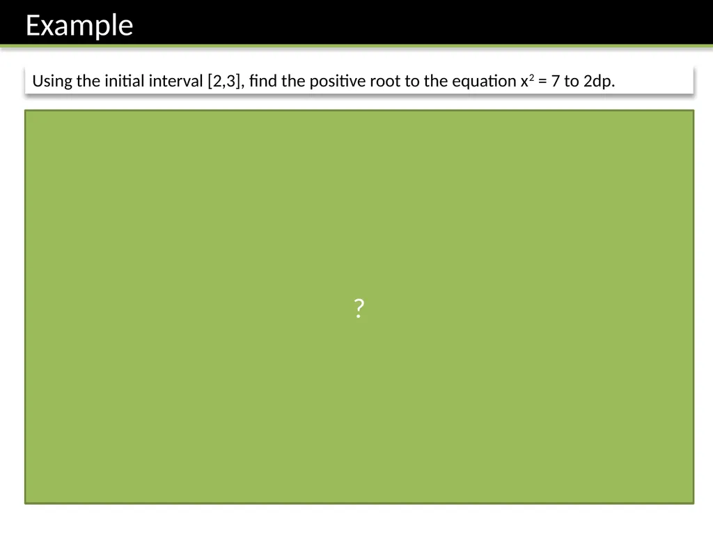
Using the initial interval [2,3], find the positive root to the equation x2 = 7 to 2dp. f(x) = x2 - 7 We can stop at this point because:
Both the new bounds will be 2.65 to 2dp, so we know the solution must be 2.65 to 2dp. ? ? Bro Tip: Keeping a table like this helps you easily keep track of your bounds. ?<br>
08
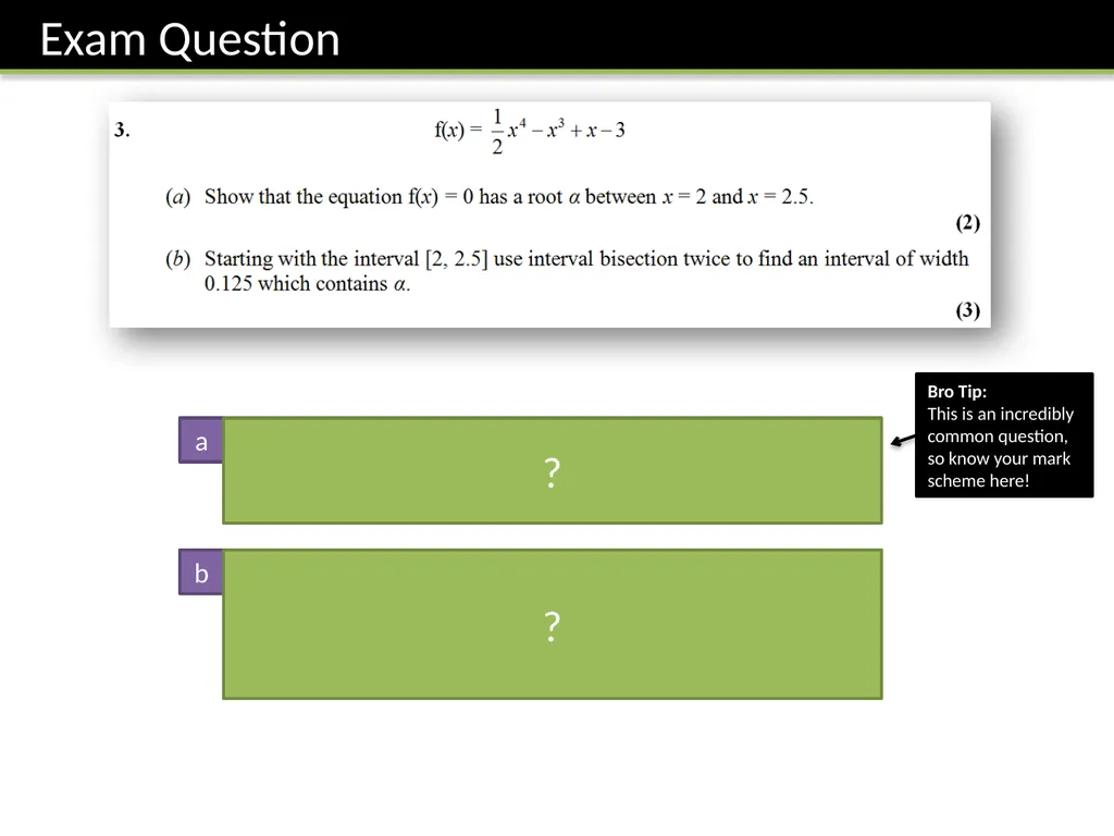
f(2) = -1, f(2.5) = 3.4062 (M1)
Sign change (and f(x) is continuous), therefore a root α exists between x = 2 and x = 2.5 (A1)
f(2.25) = 0.673828125 (B1)
f(2.125) = -0.27526855 (M1)
Therefore 2.125 α 2.25 (A1) a b ? ? Bro Tip:
This is an incredibly common question, so know your mark scheme here!<br>
10
Failure Analysis: Guaranteed to converge to a root provided that for the initial interval [a,b], f(a) and f(b) have opposite signs, and f(x) is continuous. Other Comments: Another advantage: Simple to carry out. Rate of Convergence: Horribly slow in terms of crawling very slowly towards the root. The error halves each time – we say this is linear convergence.
Therefore in practice Interval Bisection tends not to be used. (Note that none of this bit will be in an exam)<br>
11
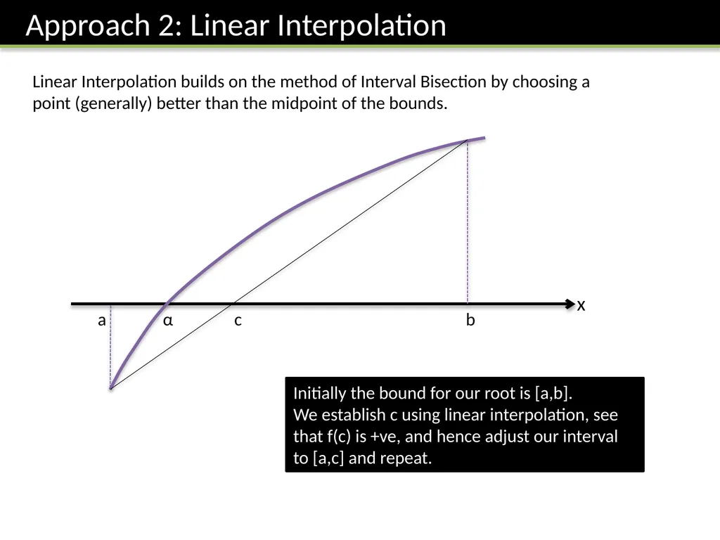
Linear Interpolation builds on the method of Interval Bisection by choosing a point (generally) better than the midpoint of the bounds. x a b α c Initially the bound for our root is [a,b].
We establish c using linear interpolation, see that f(c) is +ve, and hence adjust our interval to [a,c] and repeat.<br>
12
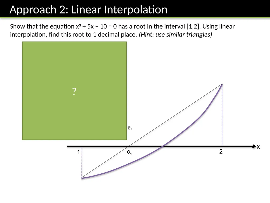
x 1 2 α1 Show that the equation x3 + 5x – 10 = 0 has a root in the interval [1,2]. Using linear interpolation, find this root to 1 decimal place. (Hint: use similar triangles) f(1) = -4, f(2) = 8
(2 – α1)/(α1 – 1) = 8/4
Solving a1 = 1.33333
f(1.333...) = -0.96296. Since negative,
Make new interval [1.333..., 2]
Eventually we find a3 = 1.4196.
We can check 1.4 is correct to 1dp by looking at f(1.35) and f(1.45). Change of sign means root root lies in [1.35, 1.45], i.e. 1.4 is correct to 1dp. ?<br>
15
Failure Analysis: As with Interval Bisection, guaranteed to converge to a root provided that for the initial interval [a,b], f(a) and f(b) have opposite signs, and f(x) is continuous. Rate of Convergence: The error of the approximation after each iteration is dependent on ‘curvy’ the line is: as you might expect, the flatter the curve is, the more it approximates a straight line, and hence the better linear interpolation will be (which assumes a straight line in the region).
The rate of convergence is high when the second derivative at the root is small (i.e. the gradient is not changing very much). (Note that none of this bit will be in an exam)<br>
16
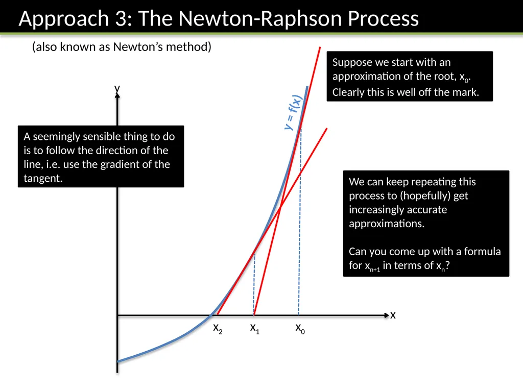
x y y = f(x) x0 Suppose we start with an approximation of the root, x0. Clearly this is well off the mark. A seemingly sensible thing to do is to follow the direction of the line, i.e. use the gradient of the tangent. x1 x2 We can keep repeating this process to (hopefully) get increasingly accurate approximations.
Can you come up with a formula for xn+1 in terms of xn? (also known as Newton’s method)<br>
17
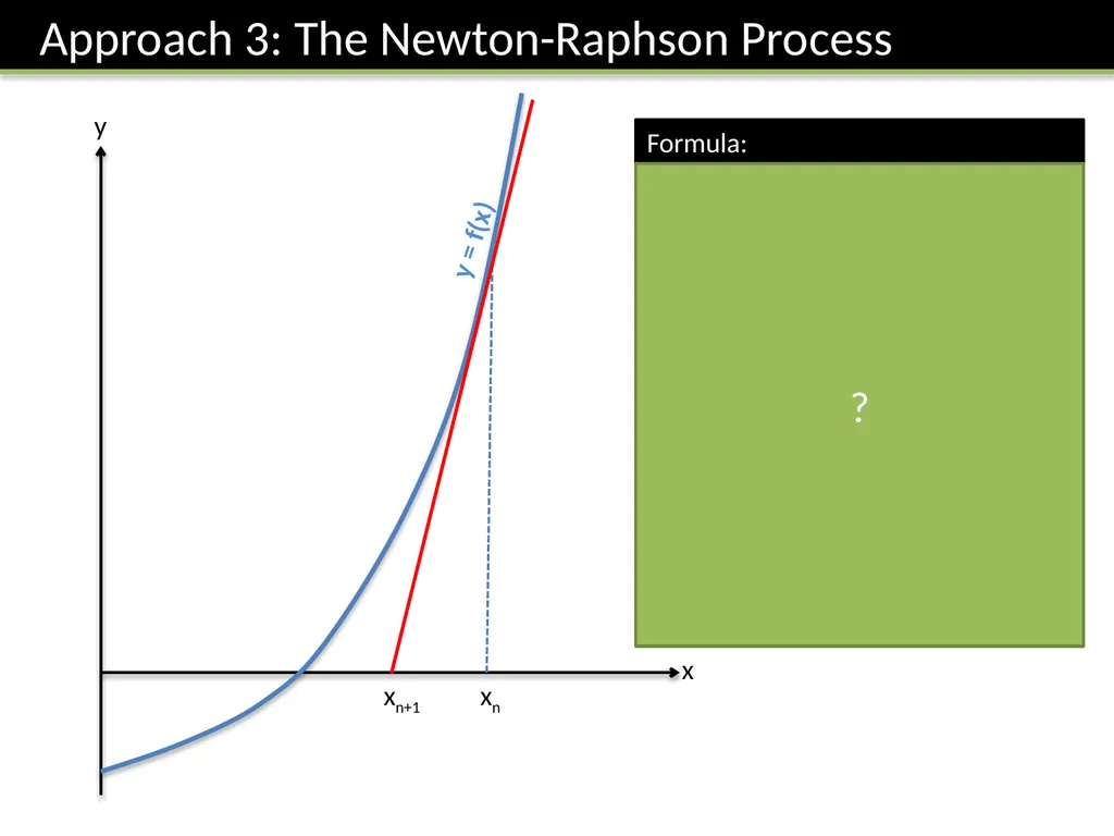
x y y = f(x) xn xn+1 Formula: Using C1 coordinate geometry:
y – f(xn) = f’(xn)(x – xn)
But we’re interested when
x = xn+1 and y = 0
-f(xn) = f’(xn)(xn+1 – xn)
which gives: Newton-Raphson Process:
xn+1 = xn - f(xn)/f’(xn) ?<br>
18
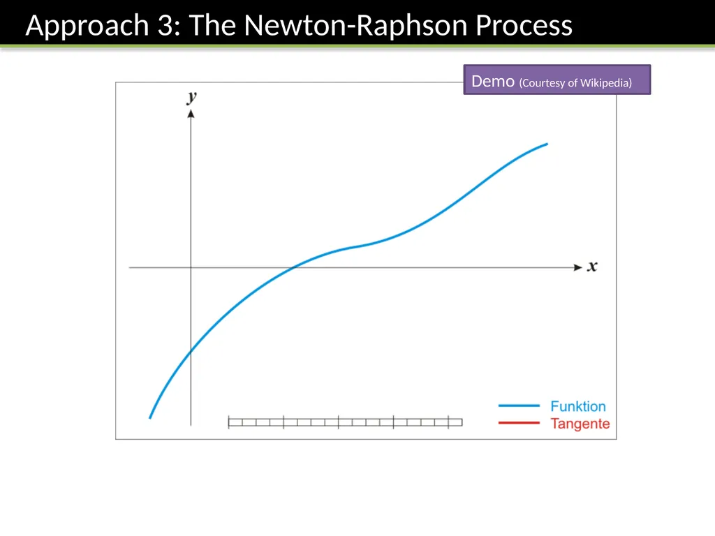
Demo (Courtesy of Wikipedia)<br>
19
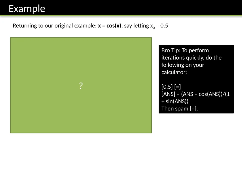
Returning to our original example: x = cos(x), say letting x0 = 0.5 Let f(x) = x – cos(x)
f’(x) = 1 + sin(x)
f(0.5) = 0.5 – cos(0.5) = -0.3775825
f’(0.5) = 1 + sin(0.5) = 1.4794255
x1 = 0.5 – (-0.3775825 / 1.4794255) = 0.7552224171
x2 = 0.7391412
x3 = 0.7390851
After merely three iterations, our approximation is accurate to 7 decimal places. Holy smokes Batman! Bro Tip: To perform iterations quickly, do the following on your calculator:
[0.5] [=]
[ANS] – (ANS – cos(ANS))/(1 + sin(ANS))
Then spam [=]. ?<br>
20
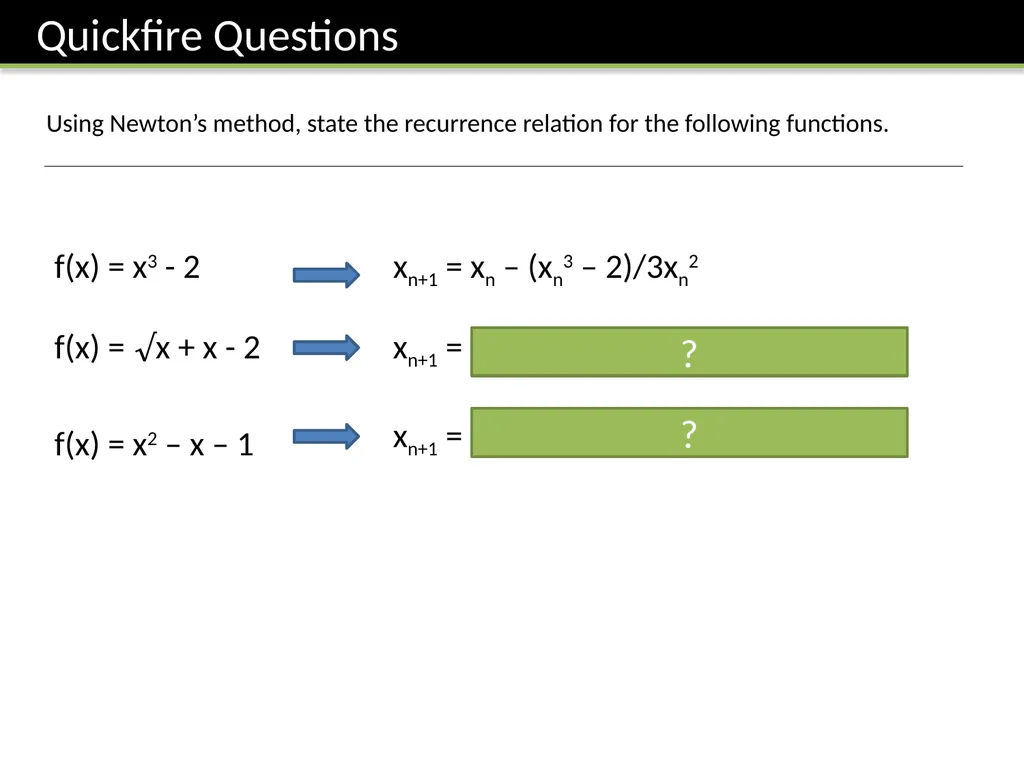
Using Newton’s method, state the recurrence relation for the following functions. f(x) = x3 - 2 xn+1 = xn – (xn3 – 2)/3xn2 f(x) = √x + x - 2 xn+1 = xn – (√xn + xn - 2)/(0.5xn-0.5 + 1) f(x) = x2 – x – 1 xn+1 = xn – (xn2 – xn – 1 )/(2xn – 1) ? ?<br>
21
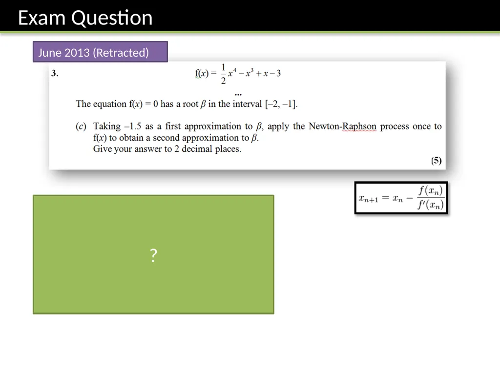
June 2013 (Retracted) f’(x) = 2x3 – 3x2 + 1
f’(-1.5) = -12.5
f(-1.5) = 1.40625
1 = -1.5 – 1.40625/(-12.5)
= -1.3875 ?<br>
23
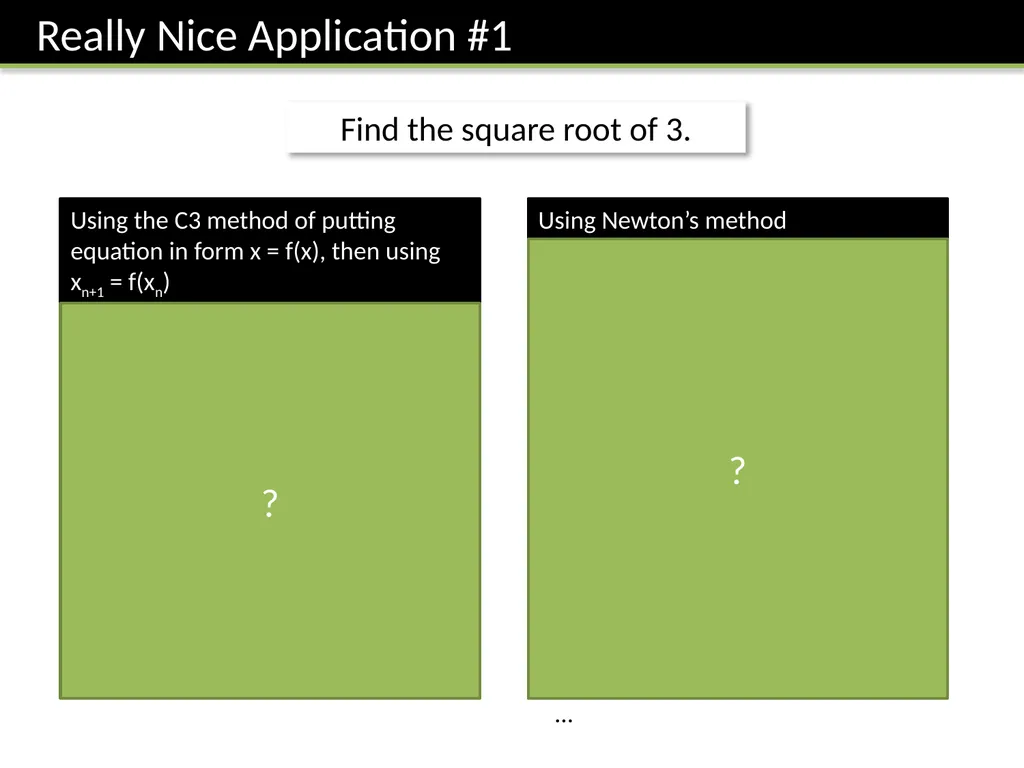
Find the square root of 3. Using the C3 method of putting equation in form x = f(x), then using xn+1 = f(xn) We want solutions to x2 = 3.
This gives xn+1 = 3/xn
This method fails to converge, because it will oscillate between two values regardless of the starting value. Using Newton’s method We want solutions to
x2 – 3 = 0
f(x) = x2 – 3
f’(x) = 2x
Using xn+1 = xn – (xn2 – 3)/2xn
x0 = 1
x1 = 2
x2 = 7/4 = 1.75
x3 = 97/56 = 1.73214
x4 = 1.73205
x5 = 1.73205
... ? ?<br>
24
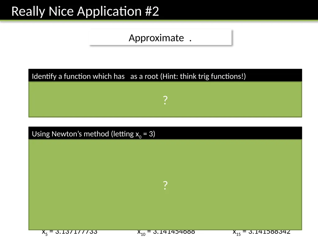
Approximate . Identify a function which has as a root (Hint: think trig functions!) Using Newton’s method (letting x0 = 3) Note that cos() = -1, so a root of f(x) = 1 + cos(x) is .
We could have also used f(x) = tan(x), provided we started between /2 and 3/2 xn+1 = xn + (1 + cos(xn))/sin(xn)
x0 = 3 (a sensible starting place!)
x1 = 3.070914844 x6 = 3.139385197 x11 = 3.141523671
x2 = 3.106268467 x7 = 3.140488926 x12 = 3.141558162
x3 = 3.123932397 x8 = 3.141040790 x13 = 3.141575408
x4 = 3.132762755 x9 = 3.141316722 x14 = 3.141584031
x5 = 3.137177733 x10 = 3.141454688 x15 = 3.141588342 ? ?<br>
25
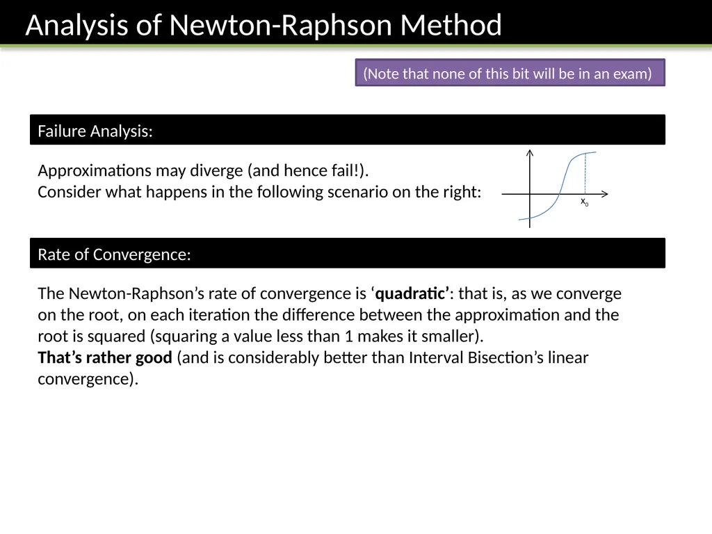
Failure Analysis: Approximations may diverge (and hence fail!).
Consider what happens in the following scenario on the right: Rate of Convergence: The Newton-Raphson’s rate of convergence is ‘quadratic’: that is, as we converge on the root, on each iteration the difference between the approximation and the root is squared (squaring a value less than 1 makes it smaller).
That’s rather good (and is considerably better than Interval Bisection’s linear convergence). (Note that none of this bit will be in an exam) x0<br>