
Frequent Itemset Mining & Association Rules Mining
TG
Published · 59 slides · 0 views
1 / 1
Description
Frequent Itemset Mining Association Rules Mining of Massive Datasets Jure Leskovec, Anand Rajaraman, Jeff Ullman Stanford University http:www.mmds.org Note to other teachers and users of these slides: We would be delighted if you found
Related Topics
Share
Embed code
Download this presentation From Below
"Frequent Itemset Mining & Association Rules Mining" is the property of its rightful owner. Permission is granted to download and print the materials on this website for personal, non-commercial use only, and to display it on your personal computer provided you do not modify the materials and that you retain all copyright notices contained in the materials. By downloading content from our website, you accept the terms of this agreement.
Presentation Transcript
01
Frequent Itemset Mining & Association Rules Mining of Massive Datasets
Jure Leskovec, Anand Rajaraman, Jeff Ullman Stanford University
http://www.mmds.org Note to other teachers and users of these slides: We would be delighted if you found this our material useful in giving your own lectures. Feel free to use these slides verbatim, or to modify them to fit your own needs. If you make use of a significant portion of these slides in your own lecture, please include this message, or a link to our web site: http://www.mmds.org<br>
Jure Leskovec, Anand Rajaraman, Jeff Ullman Stanford University
http://www.mmds.org Note to other teachers and users of these slides: We would be delighted if you found this our material useful in giving your own lectures. Feel free to use these slides verbatim, or to modify them to fit your own needs. If you make use of a significant portion of these slides in your own lecture, please include this message, or a link to our web site: http://www.mmds.org<br>
02
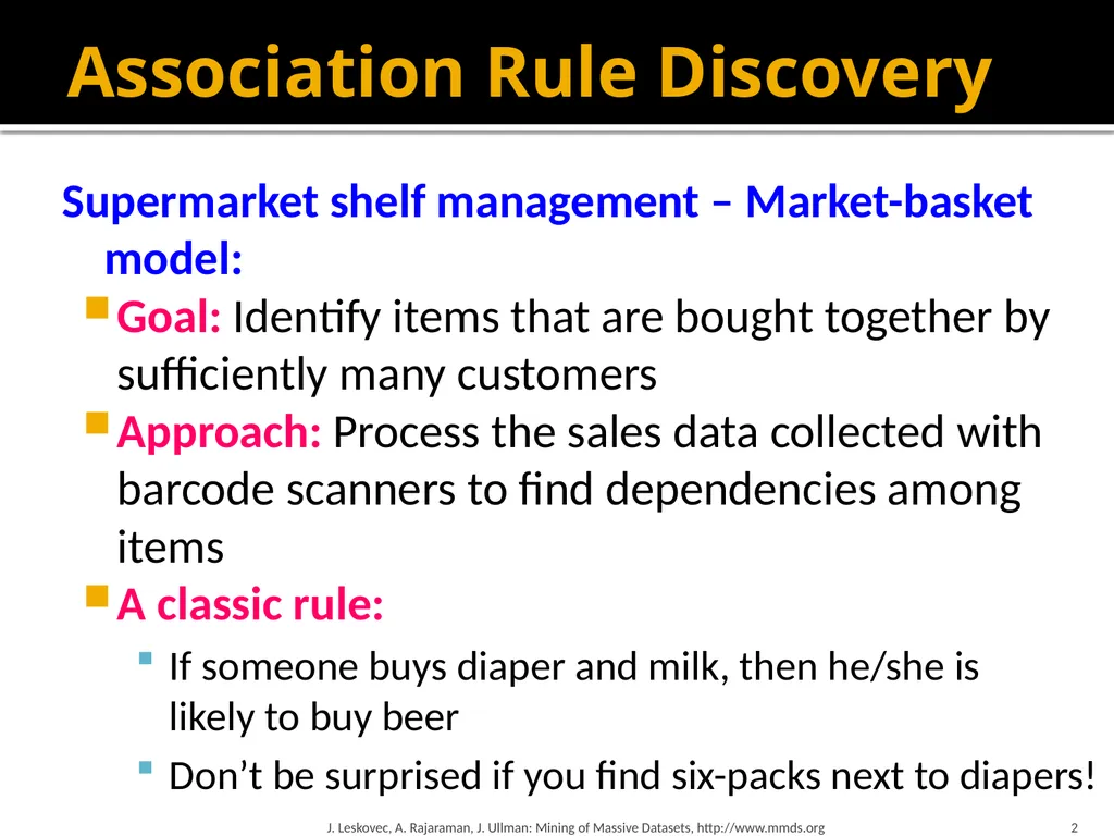
Association Rule Discovery Supermarket shelf management – Market-basket model:
Goal: Identify items that are bought together by sufficiently many customers
Approach: Process the sales data collected with barcode scanners to find dependencies among items
A classic rule:
If someone buys diaper and milk, then he/she is likely to buy beer
Don’t be surprised if you find six-packs next to diapers! J. Leskovec, A. Rajaraman, J. Ullman: Mining of Massive Datasets, http://www.mmds.org 2<br>
Goal: Identify items that are bought together by sufficiently many customers
Approach: Process the sales data collected with barcode scanners to find dependencies among items
A classic rule:
If someone buys diaper and milk, then he/she is likely to buy beer
Don’t be surprised if you find six-packs next to diapers! J. Leskovec, A. Rajaraman, J. Ullman: Mining of Massive Datasets, http://www.mmds.org 2<br>
03
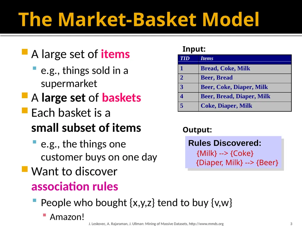
The Market-Basket Model A large set of items
e.g., things sold in a supermarket
A large set of baskets
Each basket is a small subset of items
e.g., the things one customer buys on one day
Want to discover association rules
People who bought {x,y,z} tend to buy {v,w}
Amazon! J. Leskovec, A. Rajaraman, J. Ullman: Mining of Massive Datasets, http://www.mmds.org 3 Rules Discovered:
{Milk} --> {Coke}
{Diaper, Milk} --> {Beer} Input: Output:<br>
e.g., things sold in a supermarket
A large set of baskets
Each basket is a small subset of items
e.g., the things one customer buys on one day
Want to discover association rules
People who bought {x,y,z} tend to buy {v,w}
Amazon! J. Leskovec, A. Rajaraman, J. Ullman: Mining of Massive Datasets, http://www.mmds.org 3 Rules Discovered:
{Milk} --> {Coke}
{Diaper, Milk} --> {Beer} Input: Output:<br>
04
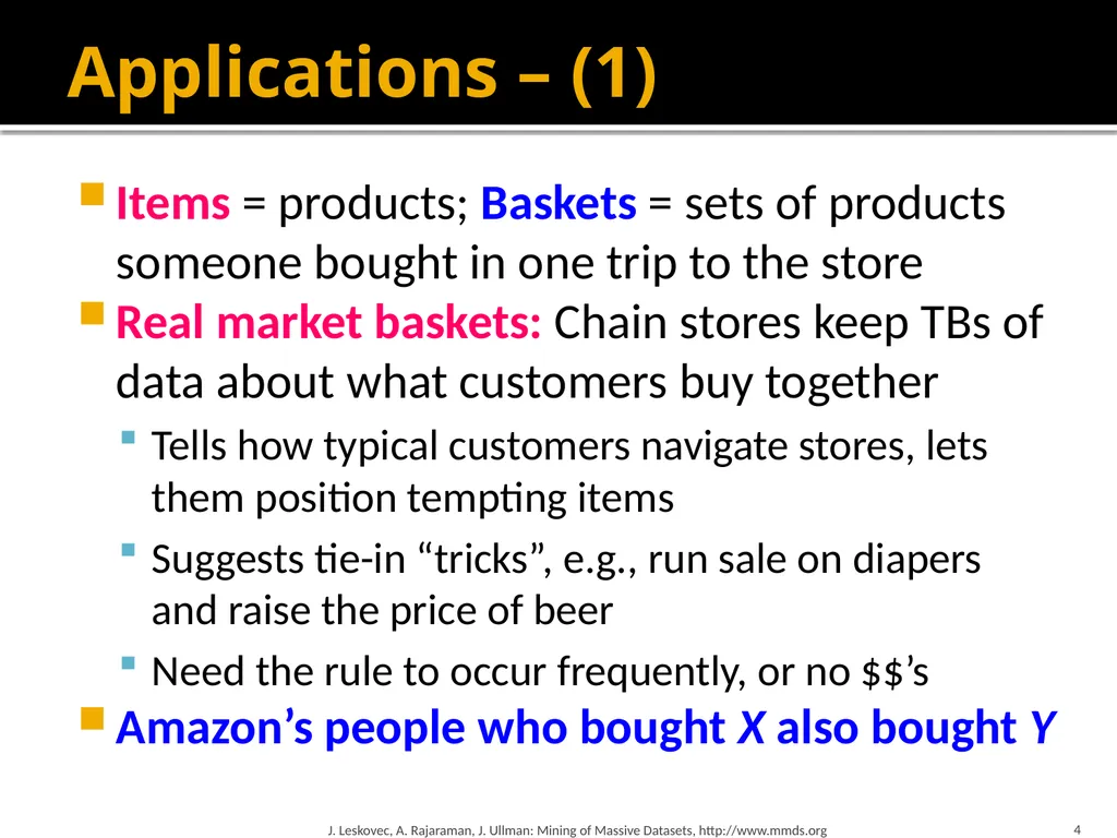
Applications – (1) Items = products; Baskets = sets of products someone bought in one trip to the store
Real market baskets: Chain stores keep TBs of data about what customers buy together
Tells how typical customers navigate stores, lets them position tempting items
Suggests tie-in “tricks”, e.g., run sale on diapers and raise the price of beer
Need the rule to occur frequently, or no $$’s
Amazon’s people who bought X also bought Y J. Leskovec, A. Rajaraman, J. Ullman: Mining of Massive Datasets, http://www.mmds.org 4<br>
Real market baskets: Chain stores keep TBs of data about what customers buy together
Tells how typical customers navigate stores, lets them position tempting items
Suggests tie-in “tricks”, e.g., run sale on diapers and raise the price of beer
Need the rule to occur frequently, or no $$’s
Amazon’s people who bought X also bought Y J. Leskovec, A. Rajaraman, J. Ullman: Mining of Massive Datasets, http://www.mmds.org 4<br>
05
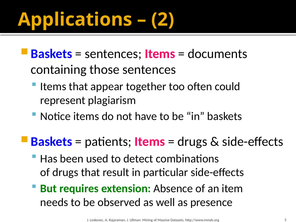
Applications – (2) Baskets = sentences; Items = documents containing those sentences
Items that appear together too often could represent plagiarism
Notice items do not have to be “in” baskets
Baskets = patients; Items = drugs & side-effects
Has been used to detect combinations of drugs that result in particular side-effects
But requires extension: Absence of an item needs to be observed as well as presence J. Leskovec, A. Rajaraman, J. Ullman: Mining of Massive Datasets, http://www.mmds.org 5<br>
Items that appear together too often could represent plagiarism
Notice items do not have to be “in” baskets
Baskets = patients; Items = drugs & side-effects
Has been used to detect combinations of drugs that result in particular side-effects
But requires extension: Absence of an item needs to be observed as well as presence J. Leskovec, A. Rajaraman, J. Ullman: Mining of Massive Datasets, http://www.mmds.org 5<br>
06
More generally A general many-to-many mapping (association) between two kinds of things
But we ask about connections among “items”, not “baskets”
For example:
Finding communities in graphs (e.g., Twitter) J. Leskovec, A. Rajaraman, J. Ullman: Mining of Massive Datasets, http://www.mmds.org 6<br>
But we ask about connections among “items”, not “baskets”
For example:
Finding communities in graphs (e.g., Twitter) J. Leskovec, A. Rajaraman, J. Ullman: Mining of Massive Datasets, http://www.mmds.org 6<br>
07
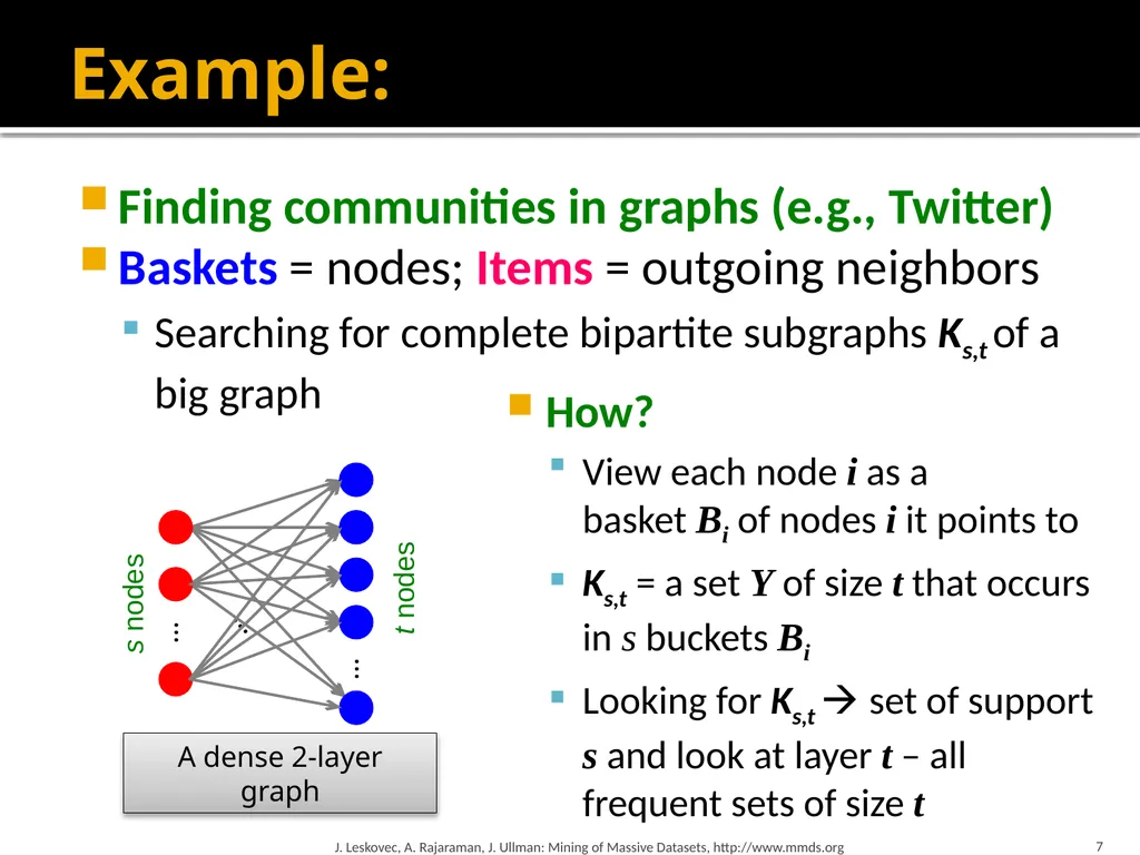
Example: Finding communities in graphs (e.g., Twitter)
Baskets = nodes; Items = outgoing neighbors
Searching for complete bipartite subgraphs Ks,t of a big graph J. Leskovec, A. Rajaraman, J. Ullman: Mining of Massive Datasets, http://www.mmds.org 7 How?
View each node i as a basket Bi of nodes i it points to
Ks,t = a set Y of size t that occurs in s buckets Bi
Looking for Ks,t set of support s and look at layer t – all frequent sets of size t … … … A dense 2-layer graph s nodes t nodes<br>
Baskets = nodes; Items = outgoing neighbors
Searching for complete bipartite subgraphs Ks,t of a big graph J. Leskovec, A. Rajaraman, J. Ullman: Mining of Massive Datasets, http://www.mmds.org 7 How?
View each node i as a basket Bi of nodes i it points to
Ks,t = a set Y of size t that occurs in s buckets Bi
Looking for Ks,t set of support s and look at layer t – all frequent sets of size t … … … A dense 2-layer graph s nodes t nodes<br>
08
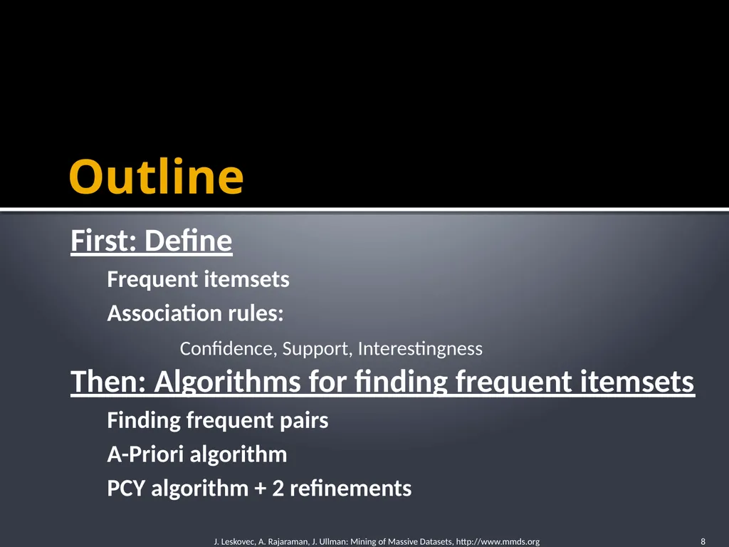
Outline First: Define
Frequent itemsets
Association rules:
Confidence, Support, Interestingness
Then: Algorithms for finding frequent itemsets
Finding frequent pairs
A-Priori algorithm
PCY algorithm + 2 refinements J. Leskovec, A. Rajaraman, J. Ullman: Mining of Massive Datasets, http://www.mmds.org 8<br>
Frequent itemsets
Association rules:
Confidence, Support, Interestingness
Then: Algorithms for finding frequent itemsets
Finding frequent pairs
A-Priori algorithm
PCY algorithm + 2 refinements J. Leskovec, A. Rajaraman, J. Ullman: Mining of Massive Datasets, http://www.mmds.org 8<br>
09
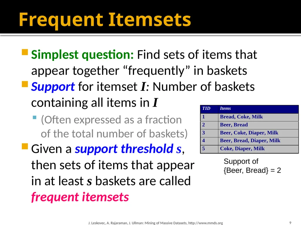
Frequent Itemsets Simplest question: Find sets of items that appear together “frequently” in baskets
Support for itemset I: Number of baskets containing all items in I
(Often expressed as a fraction of the total number of baskets)
Given a support threshold s, then sets of items that appear in at least s baskets are called frequent itemsets J. Leskovec, A. Rajaraman, J. Ullman: Mining of Massive Datasets, http://www.mmds.org 9 Support of {Beer, Bread} = 2<br>
Support for itemset I: Number of baskets containing all items in I
(Often expressed as a fraction of the total number of baskets)
Given a support threshold s, then sets of items that appear in at least s baskets are called frequent itemsets J. Leskovec, A. Rajaraman, J. Ullman: Mining of Massive Datasets, http://www.mmds.org 9 Support of {Beer, Bread} = 2<br>
10
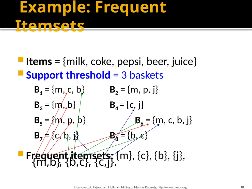
Example: Frequent Itemsets Items = {milk, coke, pepsi, beer, juice}
Support threshold = 3 baskets
B1 = {m, c, b} B2 = {m, p, j}
B3 = {m, b} B4 = {c, j}
B5 = {m, p, b} B6 = {m, c, b, j}
B7 = {c, b, j} B8 = {b, c}
Frequent itemsets: {m}, {c}, {b}, {j}, J. Leskovec, A. Rajaraman, J. Ullman: Mining of Massive Datasets, http://www.mmds.org 10<br>
Support threshold = 3 baskets
B1 = {m, c, b} B2 = {m, p, j}
B3 = {m, b} B4 = {c, j}
B5 = {m, p, b} B6 = {m, c, b, j}
B7 = {c, b, j} B8 = {b, c}
Frequent itemsets: {m}, {c}, {b}, {j}, J. Leskovec, A. Rajaraman, J. Ullman: Mining of Massive Datasets, http://www.mmds.org 10<br>
11
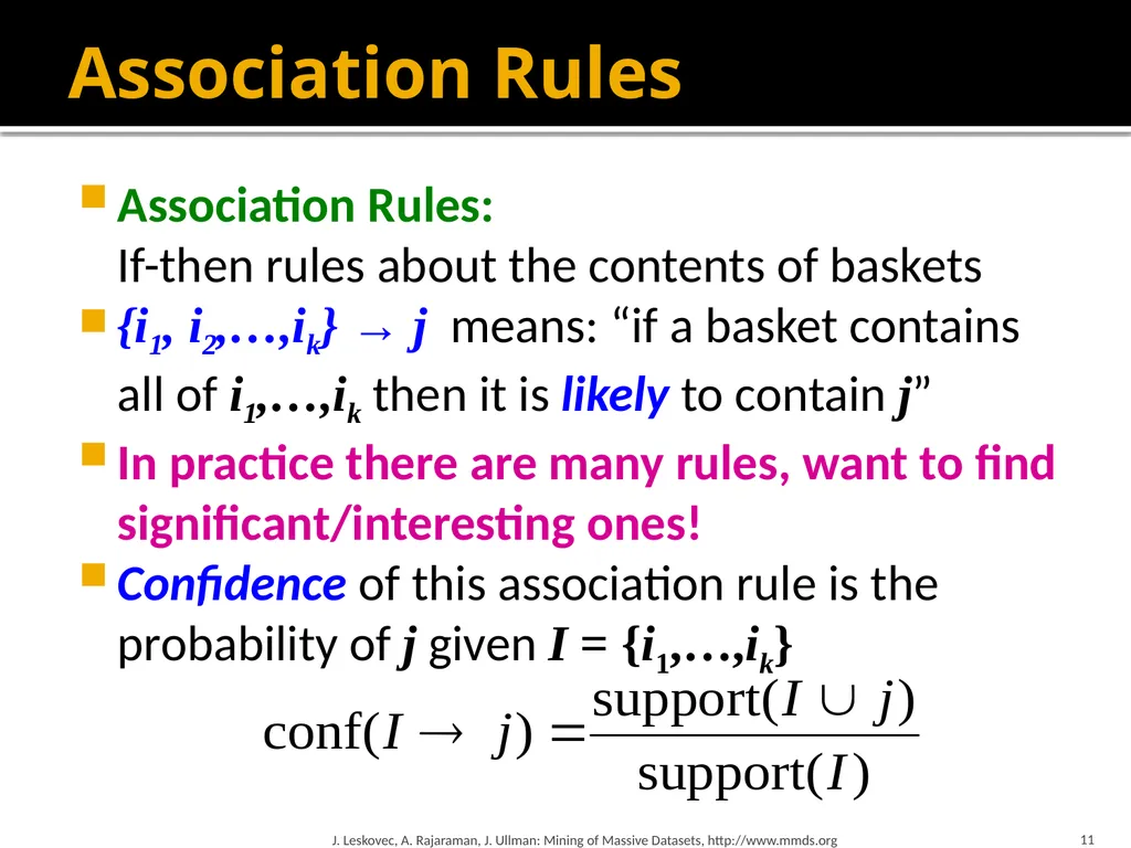
11 Association Rules Association Rules:
If-then rules about the contents of baskets
{i1, i2,…,ik} → j means: “if a basket contains all of i1,…,ik then it is likely to contain j”
In practice there are many rules, want to find significant/interesting ones!
Confidence of this association rule is the probability of j given I = {i1,…,ik} J. Leskovec, A. Rajaraman, J. Ullman: Mining of Massive Datasets, http://www.mmds.org<br>
{i1, i2,…,ik} → j means: “if a basket contains all of i1,…,ik then it is likely to contain j”
In practice there are many rules, want to find significant/interesting ones!
Confidence of this association rule is the probability of j given I = {i1,…,ik} J. Leskovec, A. Rajaraman, J. Ullman: Mining of Massive Datasets, http://www.mmds.org<br>
12
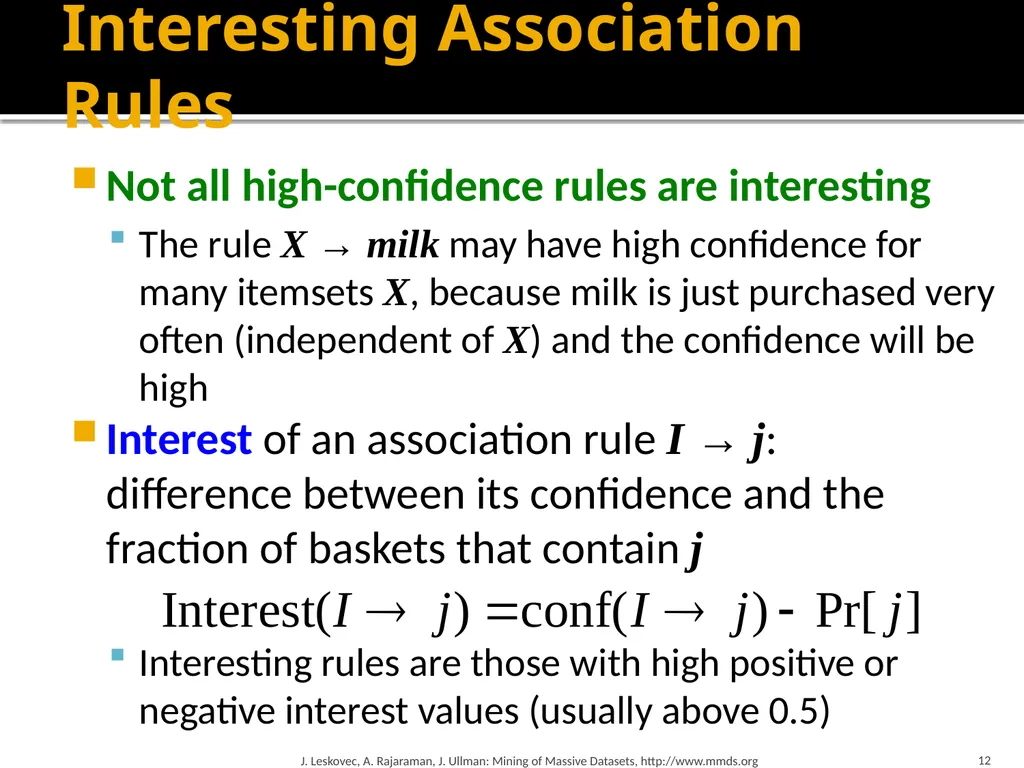
Interesting Association Rules Not all high-confidence rules are interesting
The rule X → milk may have high confidence for many itemsets X, because milk is just purchased very often (independent of X) and the confidence will be high
Interest of an association rule I → j: difference between its confidence and the fraction of baskets that contain j
Interesting rules are those with high positive or negative interest values (usually above 0.5) J. Leskovec, A. Rajaraman, J. Ullman: Mining of Massive Datasets, http://www.mmds.org 12<br>
The rule X → milk may have high confidence for many itemsets X, because milk is just purchased very often (independent of X) and the confidence will be high
Interest of an association rule I → j: difference between its confidence and the fraction of baskets that contain j
Interesting rules are those with high positive or negative interest values (usually above 0.5) J. Leskovec, A. Rajaraman, J. Ullman: Mining of Massive Datasets, http://www.mmds.org 12<br>
13
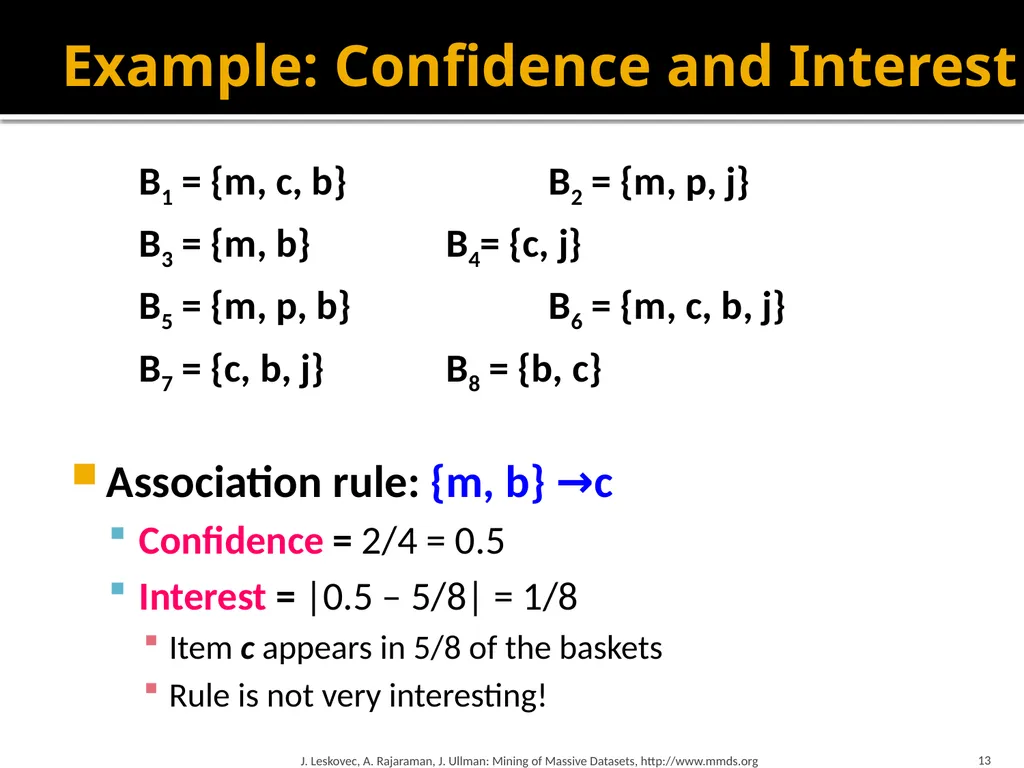
Example: Confidence and Interest B1 = {m, c, b} B2 = {m, p, j}
B3 = {m, b} B4= {c, j}
B5 = {m, p, b} B6 = {m, c, b, j}
B7 = {c, b, j} B8 = {b, c}
Association rule: {m, b} →c
Confidence = 2/4 = 0.5
Interest = |0.5 – 5/8| = 1/8
Item c appears in 5/8 of the baskets
Rule is not very interesting! J. Leskovec, A. Rajaraman, J. Ullman: Mining of Massive Datasets, http://www.mmds.org 13<br>
B3 = {m, b} B4= {c, j}
B5 = {m, p, b} B6 = {m, c, b, j}
B7 = {c, b, j} B8 = {b, c}
Association rule: {m, b} →c
Confidence = 2/4 = 0.5
Interest = |0.5 – 5/8| = 1/8
Item c appears in 5/8 of the baskets
Rule is not very interesting! J. Leskovec, A. Rajaraman, J. Ullman: Mining of Massive Datasets, http://www.mmds.org 13<br>
14
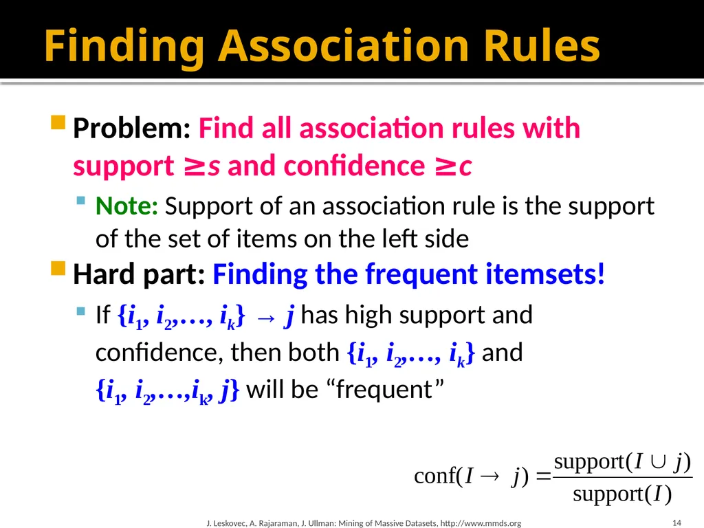
Finding Association Rules Problem: Find all association rules with support ≥s and confidence ≥c
Note: Support of an association rule is the support of the set of items on the left side
Hard part: Finding the frequent itemsets!
If {i1, i2,…, ik} → j has high support and confidence, then both {i1, i2,…, ik} and {i1, i2,…,ik, j} will be “frequent” J. Leskovec, A. Rajaraman, J. Ullman: Mining of Massive Datasets, http://www.mmds.org 14<br>
Note: Support of an association rule is the support of the set of items on the left side
Hard part: Finding the frequent itemsets!
If {i1, i2,…, ik} → j has high support and confidence, then both {i1, i2,…, ik} and {i1, i2,…,ik, j} will be “frequent” J. Leskovec, A. Rajaraman, J. Ullman: Mining of Massive Datasets, http://www.mmds.org 14<br>
15
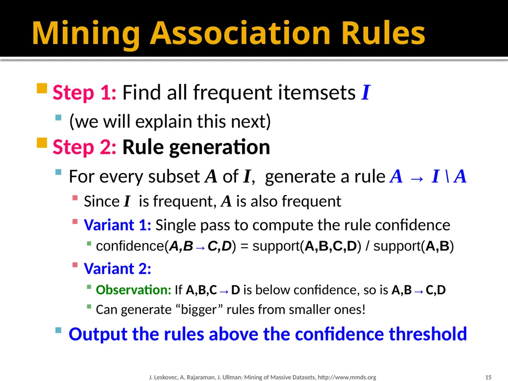
Mining Association Rules Step 1: Find all frequent itemsets I
(we will explain this next)
Step 2: Rule generation
For every subset A of I, generate a rule A → I \ A
Since I is frequent, A is also frequent
Variant 1: Single pass to compute the rule confidence
confidence(A,B→C,D) = support(A,B,C,D) / support(A,B)
Variant 2:
Observation: If A,B,C→D is below confidence, so is A,B→C,D
Can generate “bigger” rules from smaller ones!
Output the rules above the confidence threshold J. Leskovec, A. Rajaraman, J. Ullman: Mining of Massive Datasets, http://www.mmds.org 15<br>
(we will explain this next)
Step 2: Rule generation
For every subset A of I, generate a rule A → I \ A
Since I is frequent, A is also frequent
Variant 1: Single pass to compute the rule confidence
confidence(A,B→C,D) = support(A,B,C,D) / support(A,B)
Variant 2:
Observation: If A,B,C→D is below confidence, so is A,B→C,D
Can generate “bigger” rules from smaller ones!
Output the rules above the confidence threshold J. Leskovec, A. Rajaraman, J. Ullman: Mining of Massive Datasets, http://www.mmds.org 15<br>
16
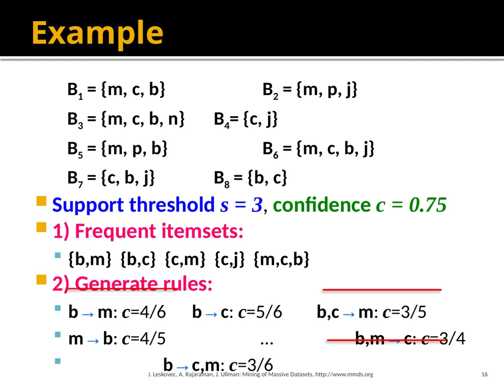
Example B1 = {m, c, b} B2 = {m, p, j}
B3 = {m, c, b, n} B4= {c, j}
B5 = {m, p, b} B6 = {m, c, b, j}
B7 = {c, b, j} B8 = {b, c}
Support threshold s = 3, confidence c = 0.75
1) Frequent itemsets:
{b,m} {b,c} {c,m} {c,j} {m,c,b}
2) Generate rules:
b→m: c=4/6 b→c: c=5/6 b,c→m: c=3/5
m→b: c=4/5 … b,m→c: c=3/4
b→c,m: c=3/6 J. Leskovec, A. Rajaraman, J. Ullman: Mining of Massive Datasets, http://www.mmds.org 16<br>
B3 = {m, c, b, n} B4= {c, j}
B5 = {m, p, b} B6 = {m, c, b, j}
B7 = {c, b, j} B8 = {b, c}
Support threshold s = 3, confidence c = 0.75
1) Frequent itemsets:
{b,m} {b,c} {c,m} {c,j} {m,c,b}
2) Generate rules:
b→m: c=4/6 b→c: c=5/6 b,c→m: c=3/5
m→b: c=4/5 … b,m→c: c=3/4
b→c,m: c=3/6 J. Leskovec, A. Rajaraman, J. Ullman: Mining of Massive Datasets, http://www.mmds.org 16<br>
17
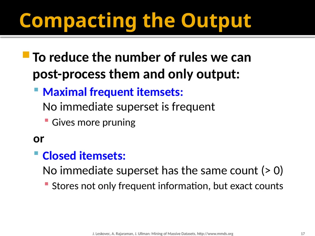
Compacting the Output To reduce the number of rules we can
post-process them and only output:
Maximal frequent itemsets: No immediate superset is frequent
Gives more pruning
or
Closed itemsets: No immediate superset has the same count (> 0)
Stores not only frequent information, but exact counts J. Leskovec, A. Rajaraman, J. Ullman: Mining of Massive Datasets, http://www.mmds.org 17<br>
Maximal frequent itemsets: No immediate superset is frequent
Gives more pruning
or
Closed itemsets: No immediate superset has the same count (> 0)
Stores not only frequent information, but exact counts J. Leskovec, A. Rajaraman, J. Ullman: Mining of Massive Datasets, http://www.mmds.org 17<br>
18
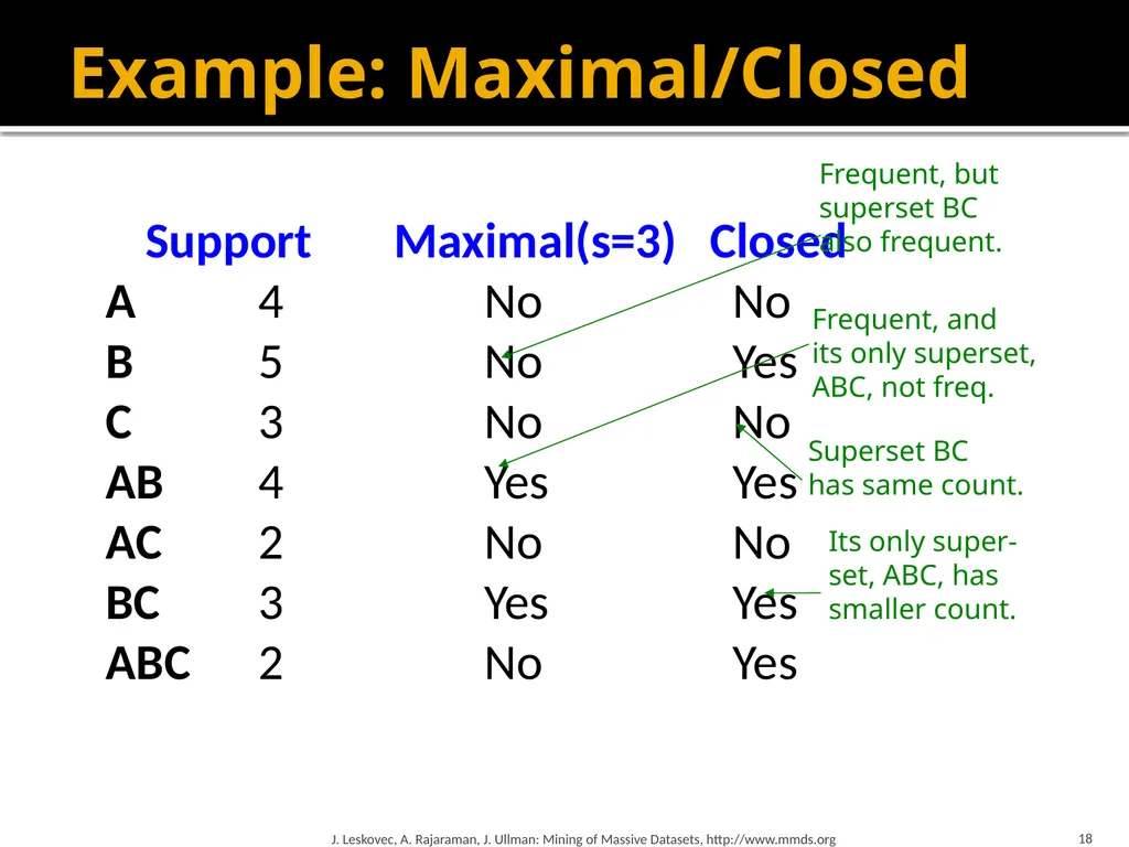
Example: Maximal/Closed Support Maximal(s=3) Closed
A 4 No No
B 5 No Yes
C 3 No No
AB 4 Yes Yes
AC 2 No No
BC 3 Yes Yes
ABC 2 No Yes J. Leskovec, A. Rajaraman, J. Ullman: Mining of Massive Datasets, http://www.mmds.org 18<br>
A 4 No No
B 5 No Yes
C 3 No No
AB 4 Yes Yes
AC 2 No No
BC 3 Yes Yes
ABC 2 No Yes J. Leskovec, A. Rajaraman, J. Ullman: Mining of Massive Datasets, http://www.mmds.org 18<br>
19
Finding Frequent Itemsets<br>
20
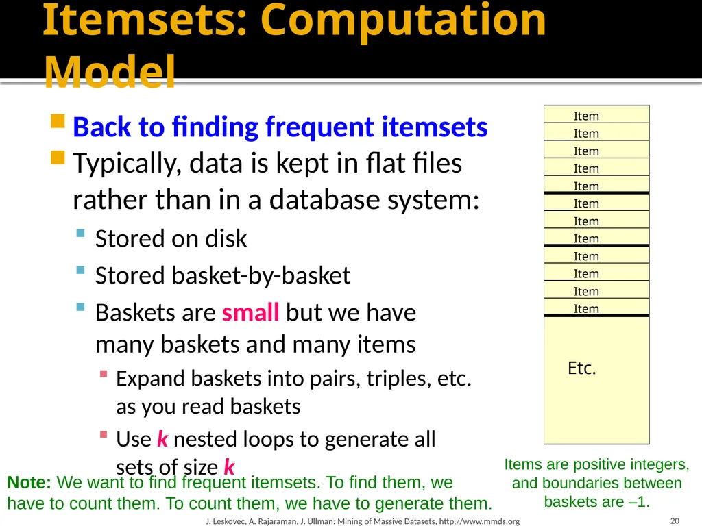
Itemsets: Computation Model Back to finding frequent itemsets
Typically, data is kept in flat files rather than in a database system:
Stored on disk
Stored basket-by-basket
Baskets are small but we have many baskets and many items
Expand baskets into pairs, triples, etc. as you read baskets
Use k nested loops to generate all sets of size k J. Leskovec, A. Rajaraman, J. Ullman: Mining of Massive Datasets, http://www.mmds.org 20 Items are positive integers, and boundaries between baskets are –1. Note: We want to find frequent itemsets. To find them, we have to count them. To count them, we have to generate them.<br>
Typically, data is kept in flat files rather than in a database system:
Stored on disk
Stored basket-by-basket
Baskets are small but we have many baskets and many items
Expand baskets into pairs, triples, etc. as you read baskets
Use k nested loops to generate all sets of size k J. Leskovec, A. Rajaraman, J. Ullman: Mining of Massive Datasets, http://www.mmds.org 20 Items are positive integers, and boundaries between baskets are –1. Note: We want to find frequent itemsets. To find them, we have to count them. To count them, we have to generate them.<br>
21
21 Computation Model The true cost of mining disk-resident data is usually the number of disk I/Os
In practice, association-rule algorithms read the data in passes – all baskets read in turn
We measure the cost by the number of passes an algorithm makes over the data J. Leskovec, A. Rajaraman, J. Ullman: Mining of Massive Datasets, http://www.mmds.org<br>
In practice, association-rule algorithms read the data in passes – all baskets read in turn
We measure the cost by the number of passes an algorithm makes over the data J. Leskovec, A. Rajaraman, J. Ullman: Mining of Massive Datasets, http://www.mmds.org<br>
22
22 Main-Memory Bottleneck For many frequent-itemset algorithms,
main-memory is the critical resource
As we read baskets, we need to count something, e.g., occurrences of pairs of items
The number of different things we can count is limited by main memory
Swapping counts in/out is a disaster (why?) J. Leskovec, A. Rajaraman, J. Ullman: Mining of Massive Datasets, http://www.mmds.org<br>
As we read baskets, we need to count something, e.g., occurrences of pairs of items
The number of different things we can count is limited by main memory
Swapping counts in/out is a disaster (why?) J. Leskovec, A. Rajaraman, J. Ullman: Mining of Massive Datasets, http://www.mmds.org<br>
23
Finding Frequent Pairs The hardest problem often turns out to be finding the frequent pairs of items {i1, i2}
Why? Freq. pairs are common, freq. triples are rare
Why? Probability of being frequent drops exponentially with size; number of sets grows more slowly with size
Let’s first concentrate on pairs, then extend to larger sets
The approach:
We always need to generate all the itemsets
But we would only like to count (keep track) of those itemsets that in the end turn out to be frequent J. Leskovec, A. Rajaraman, J. Ullman: Mining of Massive Datasets, http://www.mmds.org 23<br>
Why? Freq. pairs are common, freq. triples are rare
Why? Probability of being frequent drops exponentially with size; number of sets grows more slowly with size
Let’s first concentrate on pairs, then extend to larger sets
The approach:
We always need to generate all the itemsets
But we would only like to count (keep track) of those itemsets that in the end turn out to be frequent J. Leskovec, A. Rajaraman, J. Ullman: Mining of Massive Datasets, http://www.mmds.org 23<br>
24
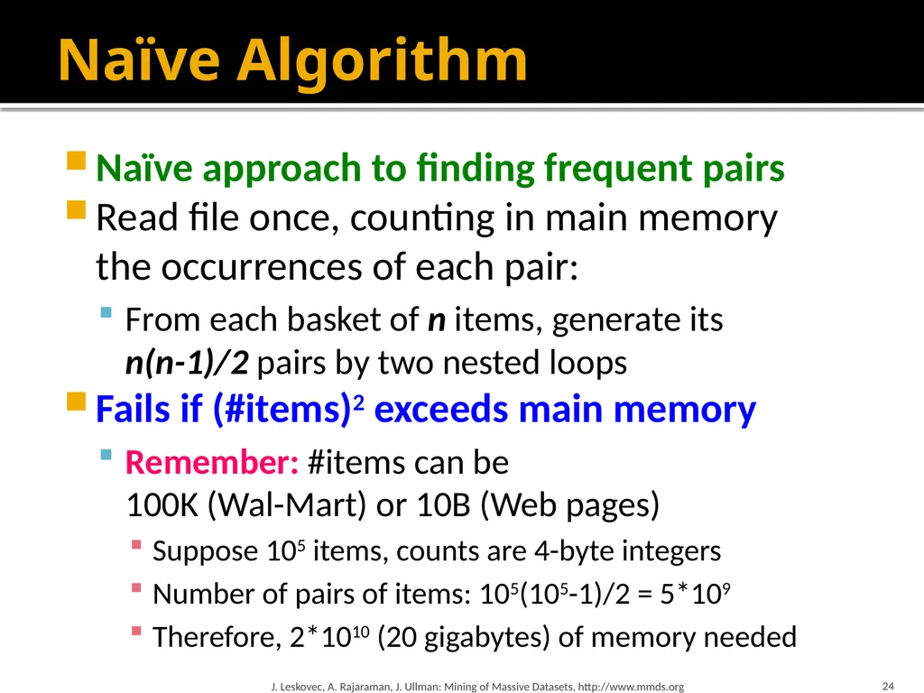
Naïve Algorithm Naïve approach to finding frequent pairs
Read file once, counting in main memory the occurrences of each pair:
From each basket of n items, generate its n(n-1)/2 pairs by two nested loops
Fails if (#items)2 exceeds main memory
Remember: #items can be 100K (Wal-Mart) or 10B (Web pages)
Suppose 105 items, counts are 4-byte integers
Number of pairs of items: 105(105-1)/2 = 5*109
Therefore, 2*1010 (20 gigabytes) of memory needed J. Leskovec, A. Rajaraman, J. Ullman: Mining of Massive Datasets, http://www.mmds.org 24<br>
Read file once, counting in main memory the occurrences of each pair:
From each basket of n items, generate its n(n-1)/2 pairs by two nested loops
Fails if (#items)2 exceeds main memory
Remember: #items can be 100K (Wal-Mart) or 10B (Web pages)
Suppose 105 items, counts are 4-byte integers
Number of pairs of items: 105(105-1)/2 = 5*109
Therefore, 2*1010 (20 gigabytes) of memory needed J. Leskovec, A. Rajaraman, J. Ullman: Mining of Massive Datasets, http://www.mmds.org 24<br>
25
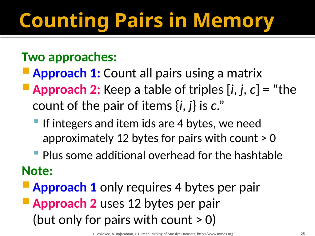
Counting Pairs in Memory Two approaches:
Approach 1: Count all pairs using a matrix
Approach 2: Keep a table of triples [i, j, c] = “the count of the pair of items {i, j} is c.”
If integers and item ids are 4 bytes, we need approximately 12 bytes for pairs with count > 0
Plus some additional overhead for the hashtable
Note:
Approach 1 only requires 4 bytes per pair
Approach 2 uses 12 bytes per pair (but only for pairs with count > 0) J. Leskovec, A. Rajaraman, J. Ullman: Mining of Massive Datasets, http://www.mmds.org 25<br>
Approach 1: Count all pairs using a matrix
Approach 2: Keep a table of triples [i, j, c] = “the count of the pair of items {i, j} is c.”
If integers and item ids are 4 bytes, we need approximately 12 bytes for pairs with count > 0
Plus some additional overhead for the hashtable
Note:
Approach 1 only requires 4 bytes per pair
Approach 2 uses 12 bytes per pair (but only for pairs with count > 0) J. Leskovec, A. Rajaraman, J. Ullman: Mining of Massive Datasets, http://www.mmds.org 25<br>
26
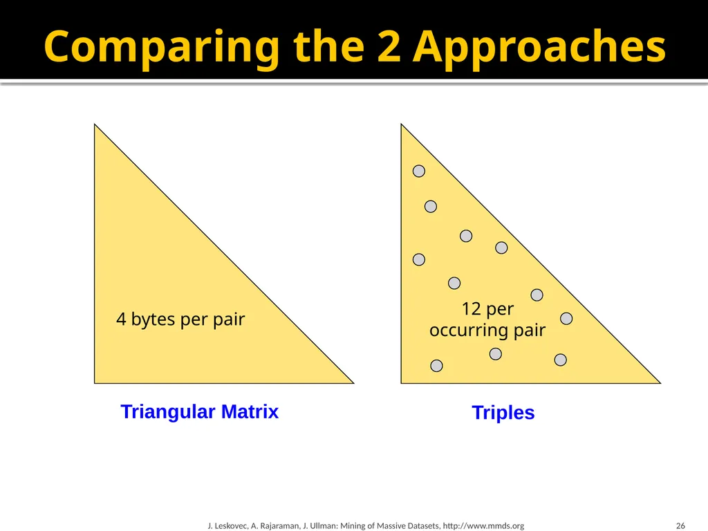
Comparing the 2 Approaches J. Leskovec, A. Rajaraman, J. Ullman: Mining of Massive Datasets, http://www.mmds.org 26 4 bytes per pair Triangular Matrix Triples 12 per
occurring pair<br>
occurring pair<br>
27
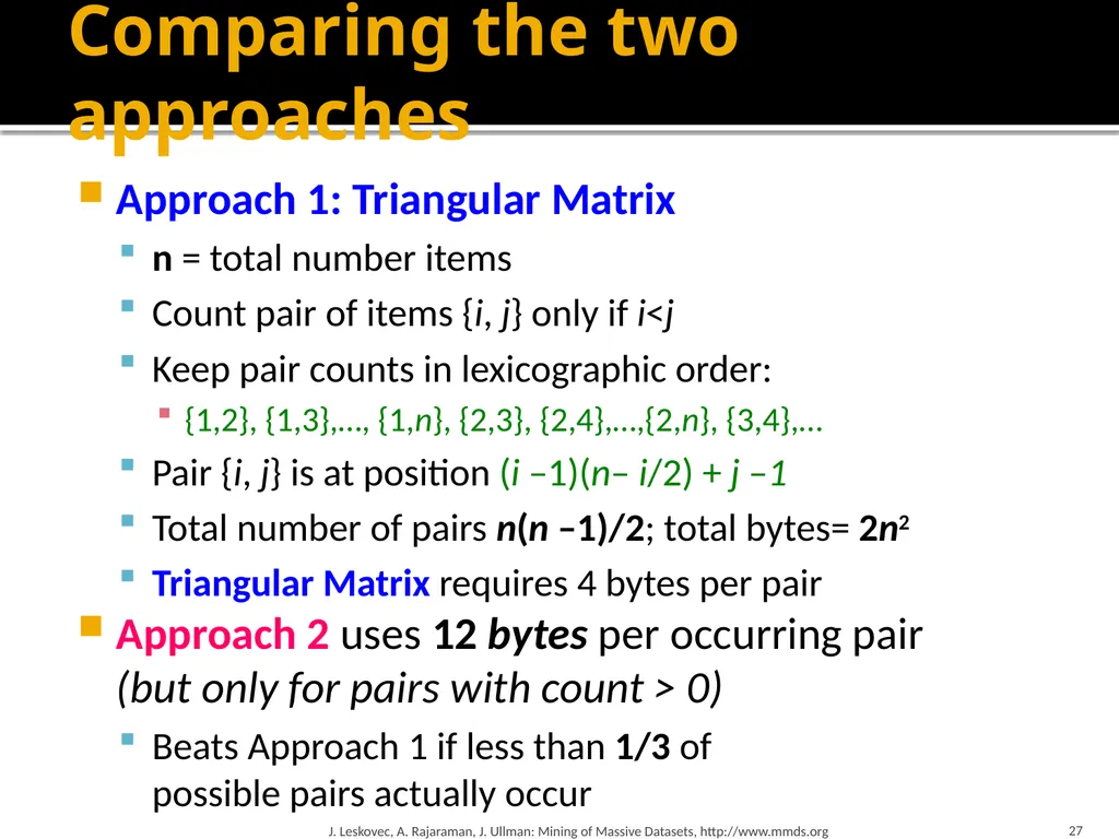
Comparing the two approaches Approach 1: Triangular Matrix
n = total number items
Count pair of items {i, j} only if i<j
Keep pair counts in lexicographic order:
{1,2}, {1,3},…, {1,n}, {2,3}, {2,4},…,{2,n}, {3,4},…
Pair {i, j} is at position (i –1)(n– i/2) + j –1
Total number of pairs n(n –1)/2; total bytes= 2n2
Triangular Matrix requires 4 bytes per pair
Approach 2 uses 12 bytes per occurring pair (but only for pairs with count > 0)
Beats Approach 1 if less than 1/3 of possible pairs actually occur J. Leskovec, A. Rajaraman, J. Ullman: Mining of Massive Datasets, http://www.mmds.org 27<br>
n = total number items
Count pair of items {i, j} only if i<j
Keep pair counts in lexicographic order:
{1,2}, {1,3},…, {1,n}, {2,3}, {2,4},…,{2,n}, {3,4},…
Pair {i, j} is at position (i –1)(n– i/2) + j –1
Total number of pairs n(n –1)/2; total bytes= 2n2
Triangular Matrix requires 4 bytes per pair
Approach 2 uses 12 bytes per occurring pair (but only for pairs with count > 0)
Beats Approach 1 if less than 1/3 of possible pairs actually occur J. Leskovec, A. Rajaraman, J. Ullman: Mining of Massive Datasets, http://www.mmds.org 27<br>
28
Comparing the two approaches Approach 1: Triangular Matrix
n = total number items
Count pair of items {i, j} only if i<j
Keep pair counts in lexicographic order:
{1,2}, {1,3},…, {1,n}, {2,3}, {2,4},…,{2,n}, {3,4},…
Pair {i, j} is at position (i –1)(n– i/2) + j –1
Total number of pairs n(n –1)/2; total bytes= 2n2
Triangular Matrix requires 4 bytes per pair
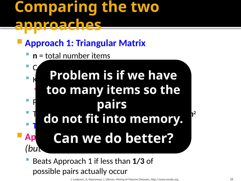
Approach 2 uses 12 bytes per pair (but only for pairs with count > 0)
Beats Approach 1 if less than 1/3 of possible pairs actually occur J. Leskovec, A. Rajaraman, J. Ullman: Mining of Massive Datasets, http://www.mmds.org 28 Problem is if we have too many items so the pairs do not fit into memory.
Can we do better?<br>
n = total number items
Count pair of items {i, j} only if i<j
Keep pair counts in lexicographic order:
{1,2}, {1,3},…, {1,n}, {2,3}, {2,4},…,{2,n}, {3,4},…
Pair {i, j} is at position (i –1)(n– i/2) + j –1
Total number of pairs n(n –1)/2; total bytes= 2n2
Triangular Matrix requires 4 bytes per pair
Approach 2 uses 12 bytes per pair (but only for pairs with count > 0)
Beats Approach 1 if less than 1/3 of possible pairs actually occur J. Leskovec, A. Rajaraman, J. Ullman: Mining of Massive Datasets, http://www.mmds.org 28 Problem is if we have too many items so the pairs do not fit into memory.
Can we do better?<br>
29
A-Priori Algorithm<br>
30
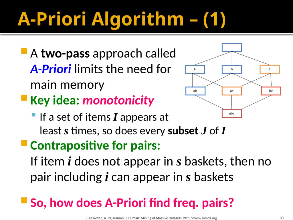
A-Priori Algorithm – (1) A two-pass approach called
A-Priori limits the need for
main memory
Key idea: monotonicity
If a set of items I appears at least s times, so does every subset J of I
Contrapositive for pairs: If item i does not appear in s baskets, then no pair including i can appear in s baskets
So, how does A-Priori find freq. pairs? J. Leskovec, A. Rajaraman, J. Ullman: Mining of Massive Datasets, http://www.mmds.org 30<br>
Key idea: monotonicity
If a set of items I appears at least s times, so does every subset J of I
Contrapositive for pairs: If item i does not appear in s baskets, then no pair including i can appear in s baskets
So, how does A-Priori find freq. pairs? J. Leskovec, A. Rajaraman, J. Ullman: Mining of Massive Datasets, http://www.mmds.org 30<br>
31
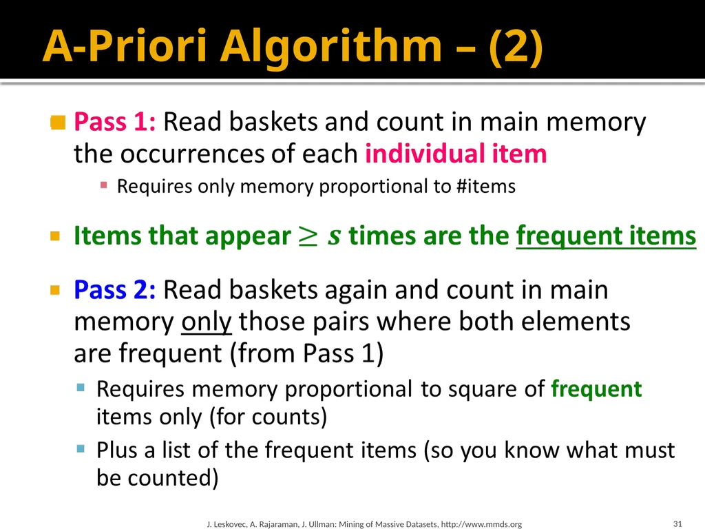
A-Priori Algorithm – (2) J. Leskovec, A. Rajaraman, J. Ullman: Mining of Massive Datasets, http://www.mmds.org 31<br>
32
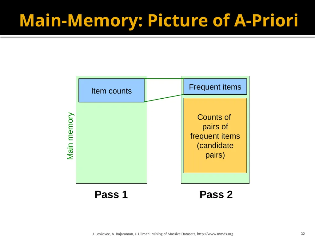
32 Main-Memory: Picture of A-Priori Item counts Pass 1 Pass 2 Frequent items J. Leskovec, A. Rajaraman, J. Ullman: Mining of Massive Datasets, http://www.mmds.org Main memory Counts of
pairs of frequent items (candidate pairs)<br>
33
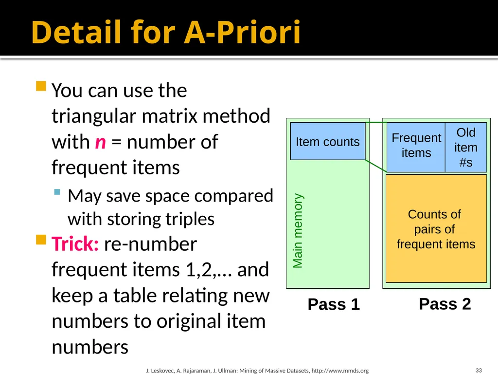
Detail for A-Priori You can use the triangular matrix method with n = number of frequent items
May save space compared with storing triples
Trick: re-number frequent items 1,2,… and keep a table relating new numbers to original item numbers J. Leskovec, A. Rajaraman, J. Ullman: Mining of Massive Datasets, http://www.mmds.org 33 Item counts Pass 1 Pass 2 Counts of pairs of frequent items Frequent items Old item #s Main memory Counts of pairs of frequent items<br>
May save space compared with storing triples
Trick: re-number frequent items 1,2,… and keep a table relating new numbers to original item numbers J. Leskovec, A. Rajaraman, J. Ullman: Mining of Massive Datasets, http://www.mmds.org 33 Item counts Pass 1 Pass 2 Counts of pairs of frequent items Frequent items Old item #s Main memory Counts of pairs of frequent items<br>
34
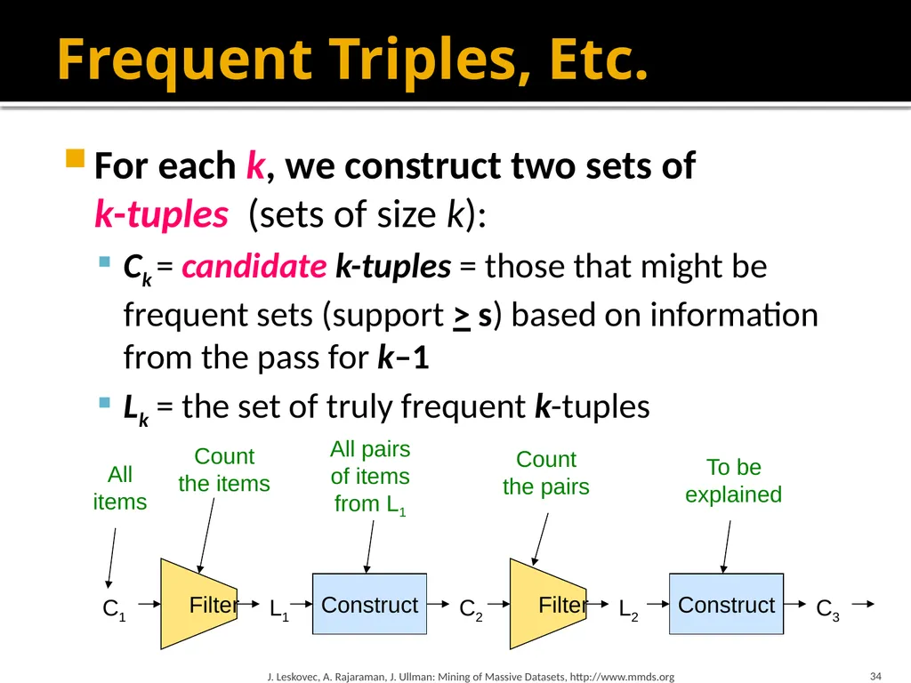
34 Frequent Triples, Etc. For each k, we construct two sets of
k-tuples (sets of size k):
Ck = candidate k-tuples = those that might be frequent sets (support > s) based on information from the pass for k–1
Lk = the set of truly frequent k-tuples J. Leskovec, A. Rajaraman, J. Ullman: Mining of Massive Datasets, http://www.mmds.org C1 L1 C2 L2 C3 Filter Filter Construct Construct<br>
Ck = candidate k-tuples = those that might be frequent sets (support > s) based on information from the pass for k–1
Lk = the set of truly frequent k-tuples J. Leskovec, A. Rajaraman, J. Ullman: Mining of Massive Datasets, http://www.mmds.org C1 L1 C2 L2 C3 Filter Filter Construct Construct<br>
35
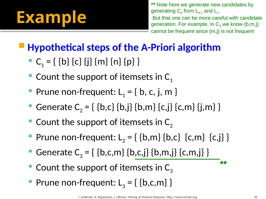
Example Hypothetical steps of the A-Priori algorithm
C1 = { {b} {c} {j} {m} {n} {p} }
Count the support of itemsets in C1
Prune non-frequent: L1 = { b, c, j, m }
Generate C2 = { {b,c} {b,j} {b,m} {c,j} {c,m} {j,m} }
Count the support of itemsets in C2
Prune non-frequent: L2 = { {b,m} {b,c} {c,m} {c,j} }
Generate C3 = { {b,c,m} {b,c,j} {b,m,j} {c,m,j} }
Count the support of itemsets in C3
Prune non-frequent: L3 = { {b,c,m} } J. Leskovec, A. Rajaraman, J. Ullman: Mining of Massive Datasets, http://www.mmds.org 35 ** Note here we generate new candidates by generating Ck from Lk-1 and L1. But that one can be more careful with candidate generation. For example, in C3 we know {b,m,j} cannot be frequent since {m,j} is not frequent **<br>
C1 = { {b} {c} {j} {m} {n} {p} }
Count the support of itemsets in C1
Prune non-frequent: L1 = { b, c, j, m }
Generate C2 = { {b,c} {b,j} {b,m} {c,j} {c,m} {j,m} }
Count the support of itemsets in C2
Prune non-frequent: L2 = { {b,m} {b,c} {c,m} {c,j} }
Generate C3 = { {b,c,m} {b,c,j} {b,m,j} {c,m,j} }
Count the support of itemsets in C3
Prune non-frequent: L3 = { {b,c,m} } J. Leskovec, A. Rajaraman, J. Ullman: Mining of Massive Datasets, http://www.mmds.org 35 ** Note here we generate new candidates by generating Ck from Lk-1 and L1. But that one can be more careful with candidate generation. For example, in C3 we know {b,m,j} cannot be frequent since {m,j} is not frequent **<br>
36
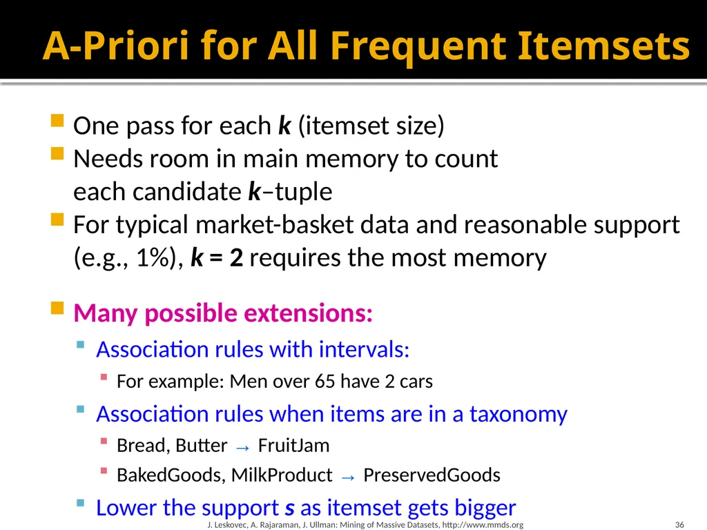
A-Priori for All Frequent Itemsets One pass for each k (itemset size)
Needs room in main memory to count each candidate k–tuple
For typical market-basket data and reasonable support (e.g., 1%), k = 2 requires the most memory
Many possible extensions:
Association rules with intervals:
For example: Men over 65 have 2 cars
Association rules when items are in a taxonomy
Bread, Butter → FruitJam
BakedGoods, MilkProduct → PreservedGoods
Lower the support s as itemset gets bigger J. Leskovec, A. Rajaraman, J. Ullman: Mining of Massive Datasets, http://www.mmds.org 36<br>
Needs room in main memory to count each candidate k–tuple
For typical market-basket data and reasonable support (e.g., 1%), k = 2 requires the most memory
Many possible extensions:
Association rules with intervals:
For example: Men over 65 have 2 cars
Association rules when items are in a taxonomy
Bread, Butter → FruitJam
BakedGoods, MilkProduct → PreservedGoods
Lower the support s as itemset gets bigger J. Leskovec, A. Rajaraman, J. Ullman: Mining of Massive Datasets, http://www.mmds.org 36<br>
37
PCY (Park-Chen-Yu) Algorithm<br>
38
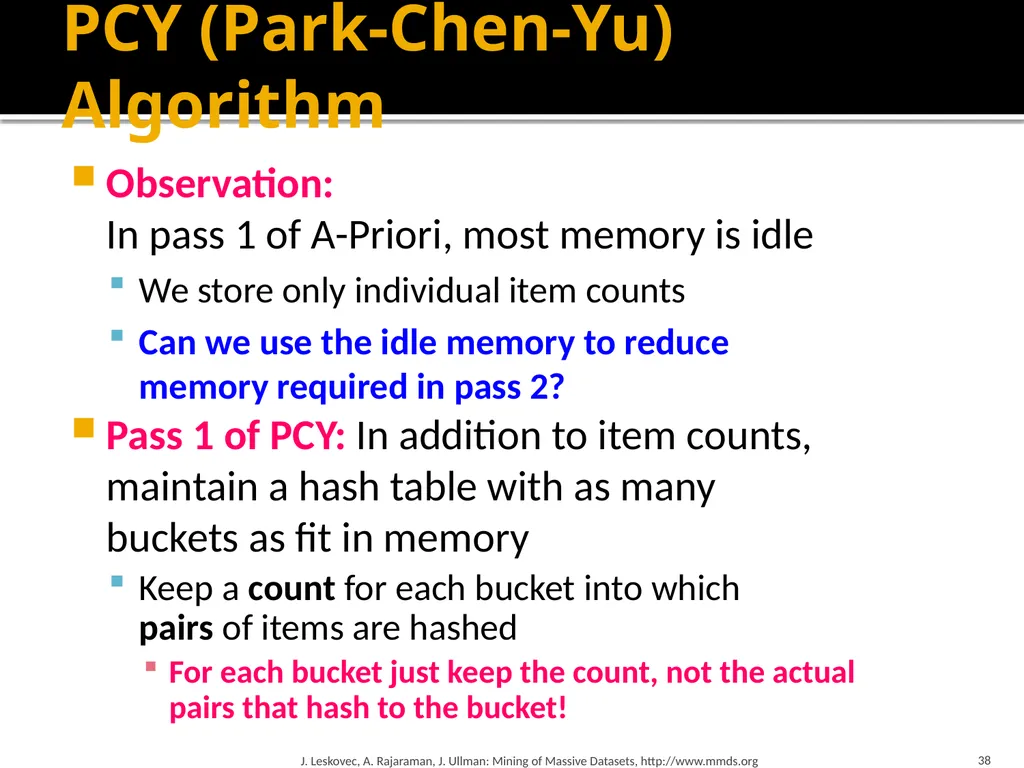
PCY (Park-Chen-Yu) Algorithm Observation:
In pass 1 of A-Priori, most memory is idle
We store only individual item counts
Can we use the idle memory to reduce memory required in pass 2?
Pass 1 of PCY: In addition to item counts, maintain a hash table with as many buckets as fit in memory
Keep a count for each bucket into which pairs of items are hashed
For each bucket just keep the count, not the actual pairs that hash to the bucket! J. Leskovec, A. Rajaraman, J. Ullman: Mining of Massive Datasets, http://www.mmds.org 38<br>
We store only individual item counts
Can we use the idle memory to reduce memory required in pass 2?
Pass 1 of PCY: In addition to item counts, maintain a hash table with as many buckets as fit in memory
Keep a count for each bucket into which pairs of items are hashed
For each bucket just keep the count, not the actual pairs that hash to the bucket! J. Leskovec, A. Rajaraman, J. Ullman: Mining of Massive Datasets, http://www.mmds.org 38<br>
39
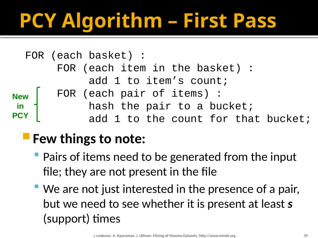
PCY Algorithm – First Pass FOR (each basket) :
FOR (each item in the basket) :
add 1 to item’s count;
FOR (each pair of items) :
hash the pair to a bucket;
add 1 to the count for that bucket;
Few things to note:
Pairs of items need to be generated from the input file; they are not present in the file
We are not just interested in the presence of a pair, but we need to see whether it is present at least s (support) times J. Leskovec, A. Rajaraman, J. Ullman: Mining of Massive Datasets, http://www.mmds.org 39 New in PCY<br>
FOR (each item in the basket) :
add 1 to item’s count;
FOR (each pair of items) :
hash the pair to a bucket;
add 1 to the count for that bucket;
Few things to note:
Pairs of items need to be generated from the input file; they are not present in the file
We are not just interested in the presence of a pair, but we need to see whether it is present at least s (support) times J. Leskovec, A. Rajaraman, J. Ullman: Mining of Massive Datasets, http://www.mmds.org 39 New in PCY<br>
40
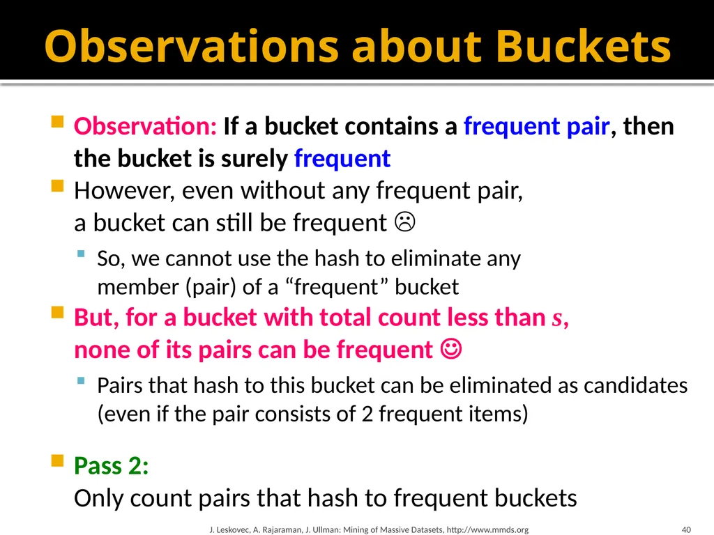
Observations about Buckets Observation: If a bucket contains a frequent pair, then the bucket is surely frequent
However, even without any frequent pair, a bucket can still be frequent
So, we cannot use the hash to eliminate any member (pair) of a “frequent” bucket
But, for a bucket with total count less than s, none of its pairs can be frequent
Pairs that hash to this bucket can be eliminated as candidates (even if the pair consists of 2 frequent items)
Pass 2: Only count pairs that hash to frequent buckets J. Leskovec, A. Rajaraman, J. Ullman: Mining of Massive Datasets, http://www.mmds.org 40<br>
However, even without any frequent pair, a bucket can still be frequent
So, we cannot use the hash to eliminate any member (pair) of a “frequent” bucket
But, for a bucket with total count less than s, none of its pairs can be frequent
Pairs that hash to this bucket can be eliminated as candidates (even if the pair consists of 2 frequent items)
Pass 2: Only count pairs that hash to frequent buckets J. Leskovec, A. Rajaraman, J. Ullman: Mining of Massive Datasets, http://www.mmds.org 40<br>
41
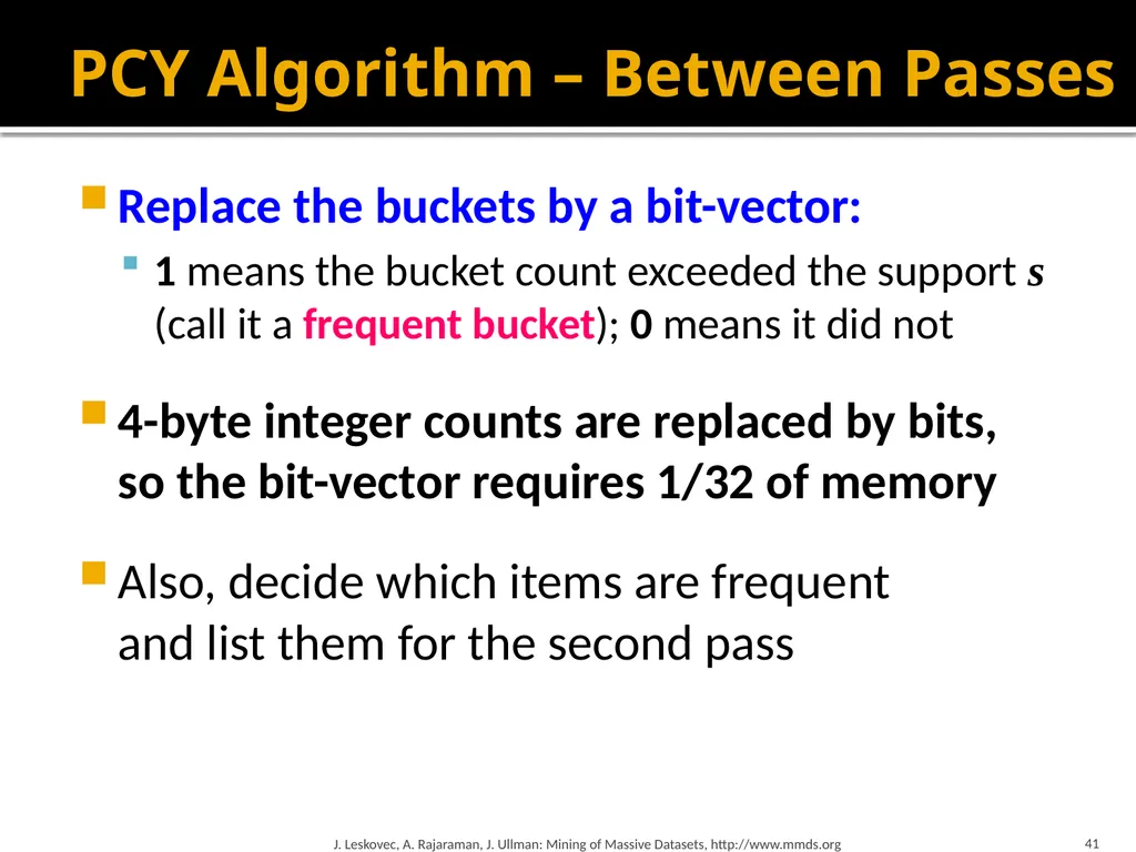
PCY Algorithm – Between Passes Replace the buckets by a bit-vector:
1 means the bucket count exceeded the support s (call it a frequent bucket); 0 means it did not
4-byte integer counts are replaced by bits, so the bit-vector requires 1/32 of memory
Also, decide which items are frequent and list them for the second pass J. Leskovec, A. Rajaraman, J. Ullman: Mining of Massive Datasets, http://www.mmds.org 41<br>
1 means the bucket count exceeded the support s (call it a frequent bucket); 0 means it did not
4-byte integer counts are replaced by bits, so the bit-vector requires 1/32 of memory
Also, decide which items are frequent and list them for the second pass J. Leskovec, A. Rajaraman, J. Ullman: Mining of Massive Datasets, http://www.mmds.org 41<br>
42
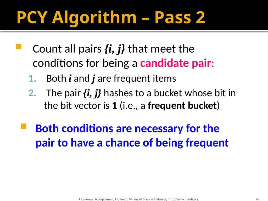
42 PCY Algorithm – Pass 2 Count all pairs {i, j} that meet the
conditions for being a candidate pair:
Both i and j are frequent items
The pair {i, j} hashes to a bucket whose bit in the bit vector is 1 (i.e., a frequent bucket)
Both conditions are necessary for the pair to have a chance of being frequent J. Leskovec, A. Rajaraman, J. Ullman: Mining of Massive Datasets, http://www.mmds.org<br>
Both i and j are frequent items
The pair {i, j} hashes to a bucket whose bit in the bit vector is 1 (i.e., a frequent bucket)
Both conditions are necessary for the pair to have a chance of being frequent J. Leskovec, A. Rajaraman, J. Ullman: Mining of Massive Datasets, http://www.mmds.org<br>
43
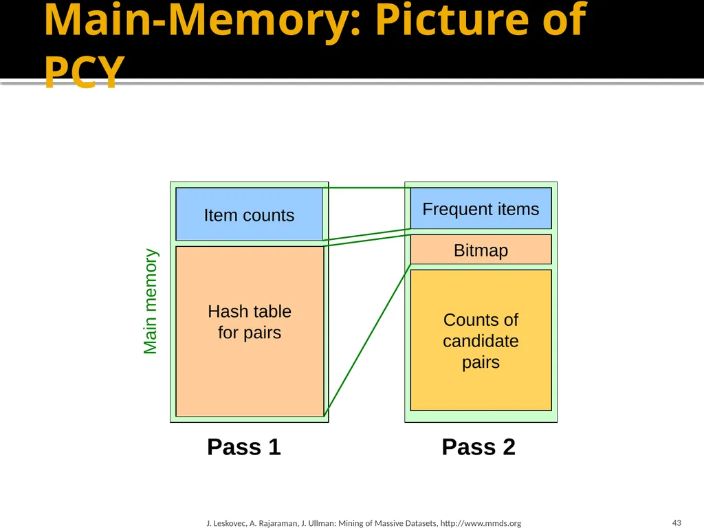
43 Main-Memory: Picture of PCY Hash
table Item counts Bitmap Pass 1 Pass 2 Frequent items J. Leskovec, A. Rajaraman, J. Ullman: Mining of Massive Datasets, http://www.mmds.org Hash table for pairs Main memory Counts of
candidate
pairs<br>
table Item counts Bitmap Pass 1 Pass 2 Frequent items J. Leskovec, A. Rajaraman, J. Ullman: Mining of Massive Datasets, http://www.mmds.org Hash table for pairs Main memory Counts of
candidate
pairs<br>
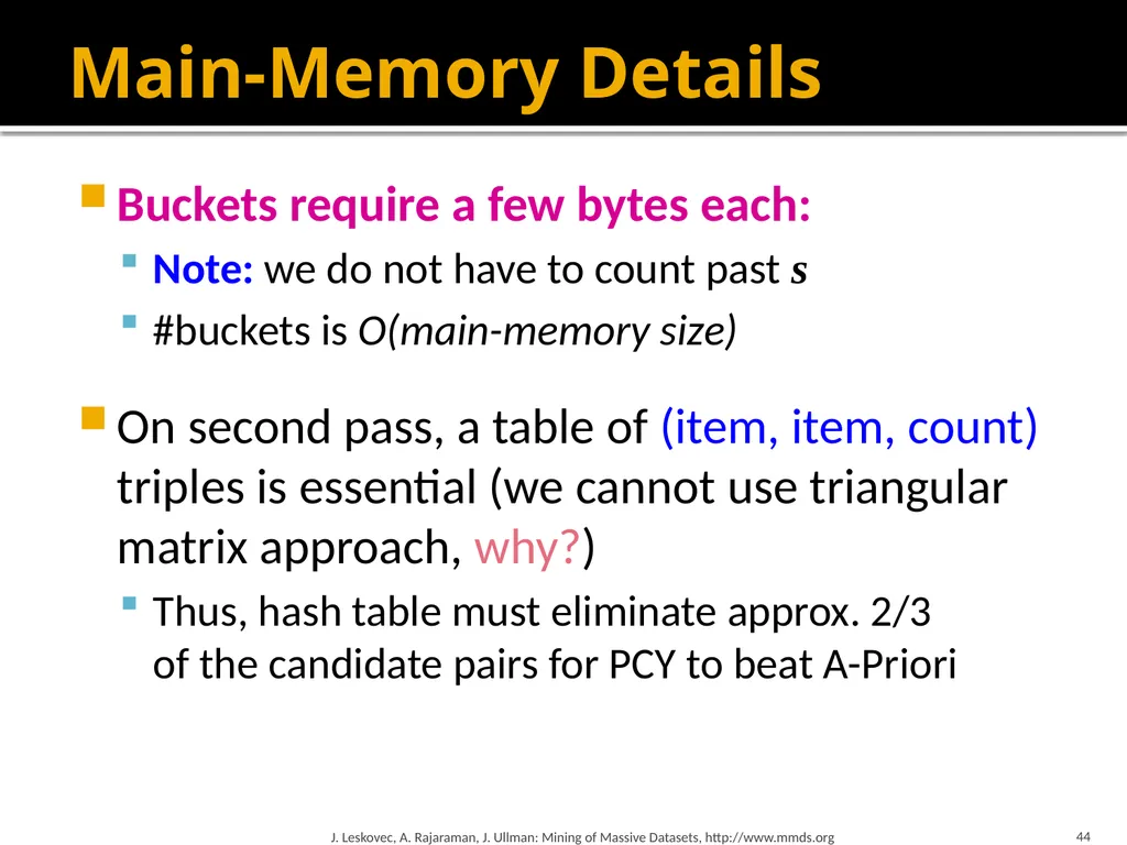
44
44 Main-Memory Details Buckets require a few bytes each:
Note: we do not have to count past s
#buckets is O(main-memory size)
On second pass, a table of (item, item, count) triples is essential (we cannot use triangular matrix approach, why?)
Thus, hash table must eliminate approx. 2/3 of the candidate pairs for PCY to beat A-Priori J. Leskovec, A. Rajaraman, J. Ullman: Mining of Massive Datasets, http://www.mmds.org<br>
Note: we do not have to count past s
#buckets is O(main-memory size)
On second pass, a table of (item, item, count) triples is essential (we cannot use triangular matrix approach, why?)
Thus, hash table must eliminate approx. 2/3 of the candidate pairs for PCY to beat A-Priori J. Leskovec, A. Rajaraman, J. Ullman: Mining of Massive Datasets, http://www.mmds.org<br>
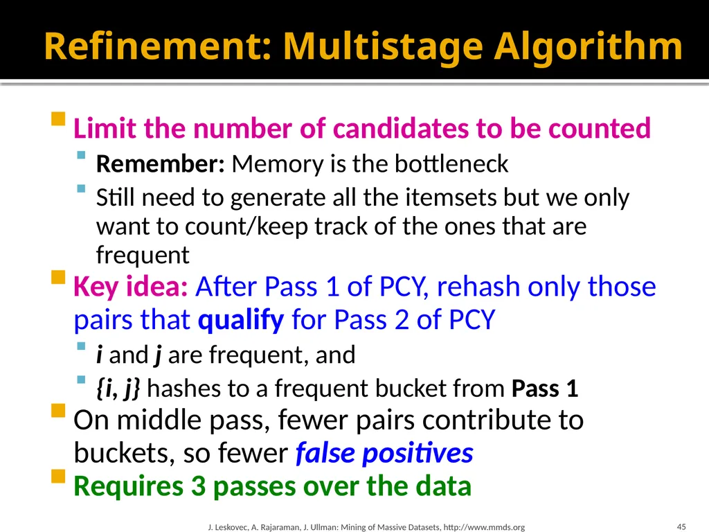
45
Refinement: Multistage Algorithm Limit the number of candidates to be counted
Remember: Memory is the bottleneck
Still need to generate all the itemsets but we only want to count/keep track of the ones that are frequent
Key idea: After Pass 1 of PCY, rehash only those pairs that qualify for Pass 2 of PCY
i and j are frequent, and
{i, j} hashes to a frequent bucket from Pass 1
On middle pass, fewer pairs contribute to buckets, so fewer false positives
Requires 3 passes over the data J. Leskovec, A. Rajaraman, J. Ullman: Mining of Massive Datasets, http://www.mmds.org 45<br>
Remember: Memory is the bottleneck
Still need to generate all the itemsets but we only want to count/keep track of the ones that are frequent
Key idea: After Pass 1 of PCY, rehash only those pairs that qualify for Pass 2 of PCY
i and j are frequent, and
{i, j} hashes to a frequent bucket from Pass 1
On middle pass, fewer pairs contribute to buckets, so fewer false positives
Requires 3 passes over the data J. Leskovec, A. Rajaraman, J. Ullman: Mining of Massive Datasets, http://www.mmds.org 45<br>
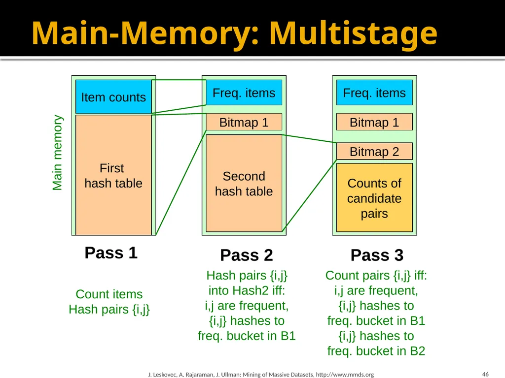
46
46 Main-Memory: Multistage First
hash table Item counts Bitmap 1 Bitmap 1 Bitmap 2 Freq. items Freq. items Counts of
candidate
pairs Pass 1 Pass 2 Pass 3 J. Leskovec, A. Rajaraman, J. Ullman: Mining of Massive Datasets, http://www.mmds.org Count items
Hash pairs {i,j} Hash pairs {i,j} into Hash2 iff:
i,j are frequent, {i,j} hashes to
freq. bucket in B1 Count pairs {i,j} iff:
i,j are frequent, {i,j} hashes to
freq. bucket in B1
{i,j} hashes to
freq. bucket in B2 First hash table Second hash table Counts of
candidate
pairs Main memory<br>
hash table Item counts Bitmap 1 Bitmap 1 Bitmap 2 Freq. items Freq. items Counts of
candidate
pairs Pass 1 Pass 2 Pass 3 J. Leskovec, A. Rajaraman, J. Ullman: Mining of Massive Datasets, http://www.mmds.org Count items
Hash pairs {i,j} Hash pairs {i,j} into Hash2 iff:
i,j are frequent, {i,j} hashes to
freq. bucket in B1 Count pairs {i,j} iff:
i,j are frequent, {i,j} hashes to
freq. bucket in B1
{i,j} hashes to
freq. bucket in B2 First hash table Second hash table Counts of
candidate
pairs Main memory<br>
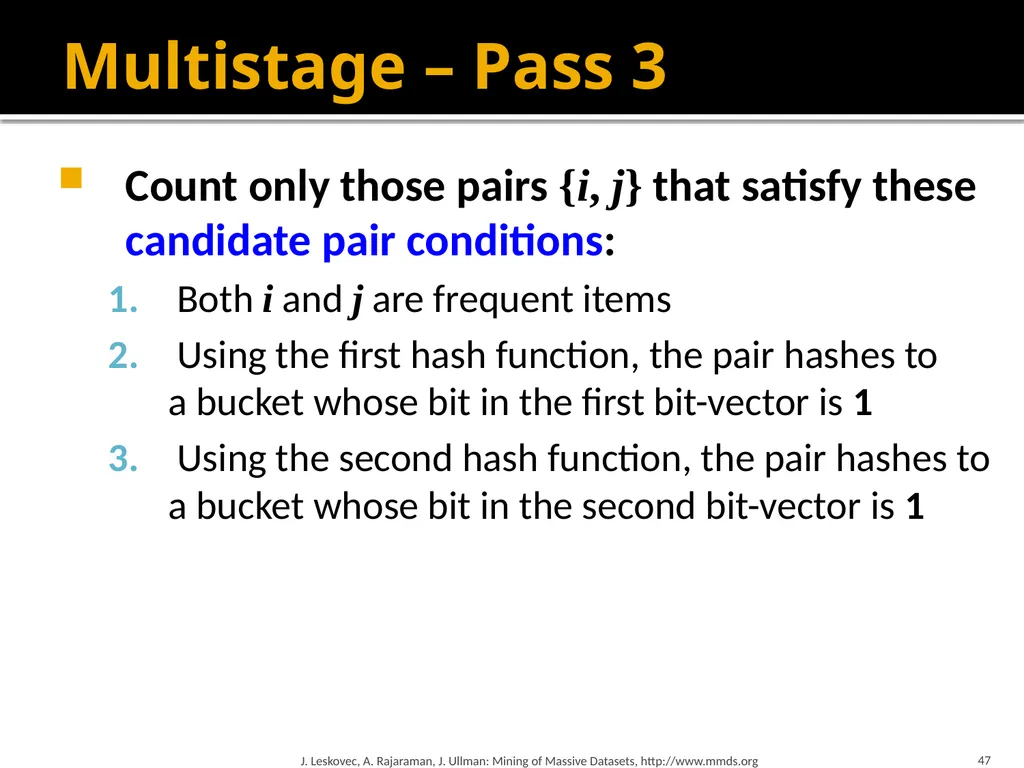
47
Multistage – Pass 3 Count only those pairs {i, j} that satisfy these candidate pair conditions:
Both i and j are frequent items
Using the first hash function, the pair hashes to a bucket whose bit in the first bit-vector is 1
Using the second hash function, the pair hashes to a bucket whose bit in the second bit-vector is 1 J. Leskovec, A. Rajaraman, J. Ullman: Mining of Massive Datasets, http://www.mmds.org 47<br>
Both i and j are frequent items
Using the first hash function, the pair hashes to a bucket whose bit in the first bit-vector is 1
Using the second hash function, the pair hashes to a bucket whose bit in the second bit-vector is 1 J. Leskovec, A. Rajaraman, J. Ullman: Mining of Massive Datasets, http://www.mmds.org 47<br>
48
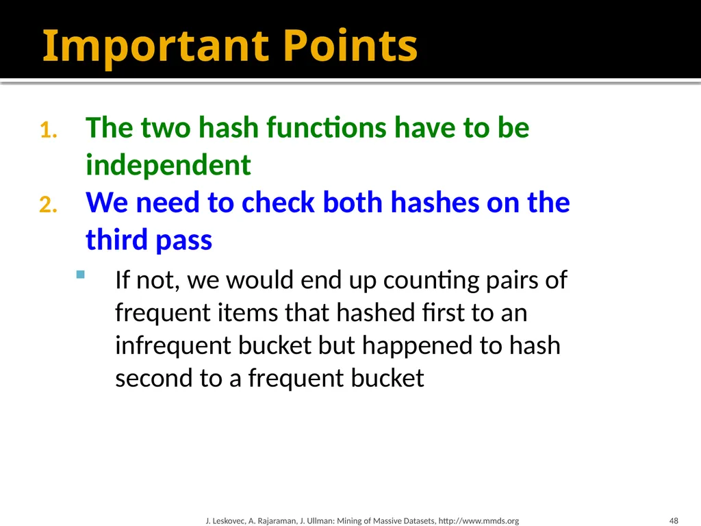
Important Points The two hash functions have to be independent
We need to check both hashes on the third pass
If not, we would end up counting pairs of frequent items that hashed first to an infrequent bucket but happened to hash second to a frequent bucket J. Leskovec, A. Rajaraman, J. Ullman: Mining of Massive Datasets, http://www.mmds.org 48<br>
We need to check both hashes on the third pass
If not, we would end up counting pairs of frequent items that hashed first to an infrequent bucket but happened to hash second to a frequent bucket J. Leskovec, A. Rajaraman, J. Ullman: Mining of Massive Datasets, http://www.mmds.org 48<br>
49
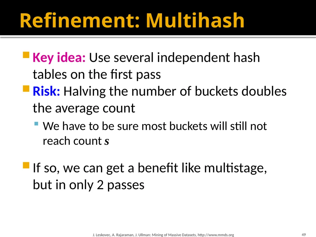
Refinement: Multihash Key idea: Use several independent hash tables on the first pass
Risk: Halving the number of buckets doubles the average count
We have to be sure most buckets will still not reach count s
If so, we can get a benefit like multistage, but in only 2 passes J. Leskovec, A. Rajaraman, J. Ullman: Mining of Massive Datasets, http://www.mmds.org 49<br>
Risk: Halving the number of buckets doubles the average count
We have to be sure most buckets will still not reach count s
If so, we can get a benefit like multistage, but in only 2 passes J. Leskovec, A. Rajaraman, J. Ullman: Mining of Massive Datasets, http://www.mmds.org 49<br>
50
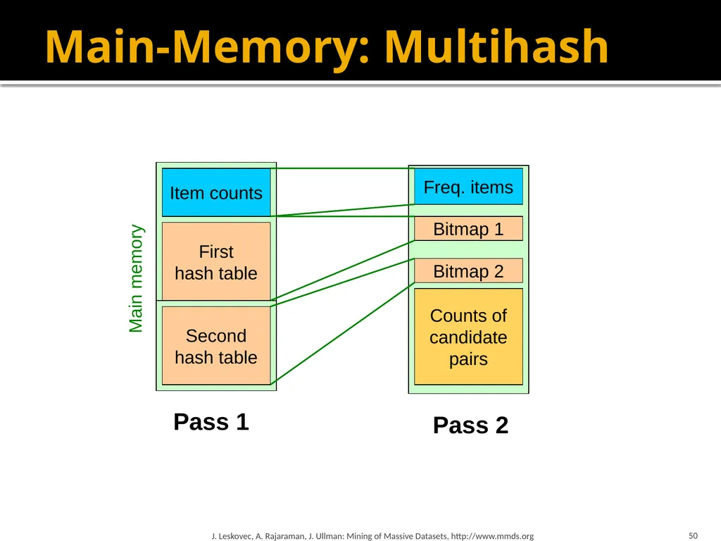
Main-Memory: Multihash J. Leskovec, A. Rajaraman, J. Ullman: Mining of Massive Datasets, http://www.mmds.org 50 First hash
table
Second
hash table Item counts Pass 1 Pass 2 First hash table Second hash table Counts of
candidate
pairs Main memory<br>
table
Second
hash table Item counts Pass 1 Pass 2 First hash table Second hash table Counts of
candidate
pairs Main memory<br>
51
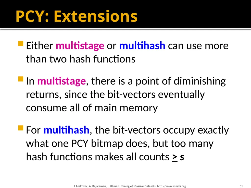
PCY: Extensions Either multistage or multihash can use more than two hash functions
In multistage, there is a point of diminishing returns, since the bit-vectors eventually consume all of main memory
For multihash, the bit-vectors occupy exactly what one PCY bitmap does, but too many hash functions makes all counts > s 51 J. Leskovec, A. Rajaraman, J. Ullman: Mining of Massive Datasets, http://www.mmds.org<br>
In multistage, there is a point of diminishing returns, since the bit-vectors eventually consume all of main memory
For multihash, the bit-vectors occupy exactly what one PCY bitmap does, but too many hash functions makes all counts > s 51 J. Leskovec, A. Rajaraman, J. Ullman: Mining of Massive Datasets, http://www.mmds.org<br>
52
Frequent Itemsets
in < 2 Passes<br>
53
Frequent Itemsets in < 2 Passes A-Priori, PCY, etc., take k passes to find frequent itemsets of size k
Can we use fewer passes?
Use 2 or fewer passes for all sizes, but may miss some frequent itemsets
Random sampling
SON (Savasere, Omiecinski, and Navathe)
Toivonen (see textbook) J. Leskovec, A. Rajaraman, J. Ullman: Mining of Massive Datasets, http://www.mmds.org 53<br>
Can we use fewer passes?
Use 2 or fewer passes for all sizes, but may miss some frequent itemsets
Random sampling
SON (Savasere, Omiecinski, and Navathe)
Toivonen (see textbook) J. Leskovec, A. Rajaraman, J. Ullman: Mining of Massive Datasets, http://www.mmds.org 53<br>
54
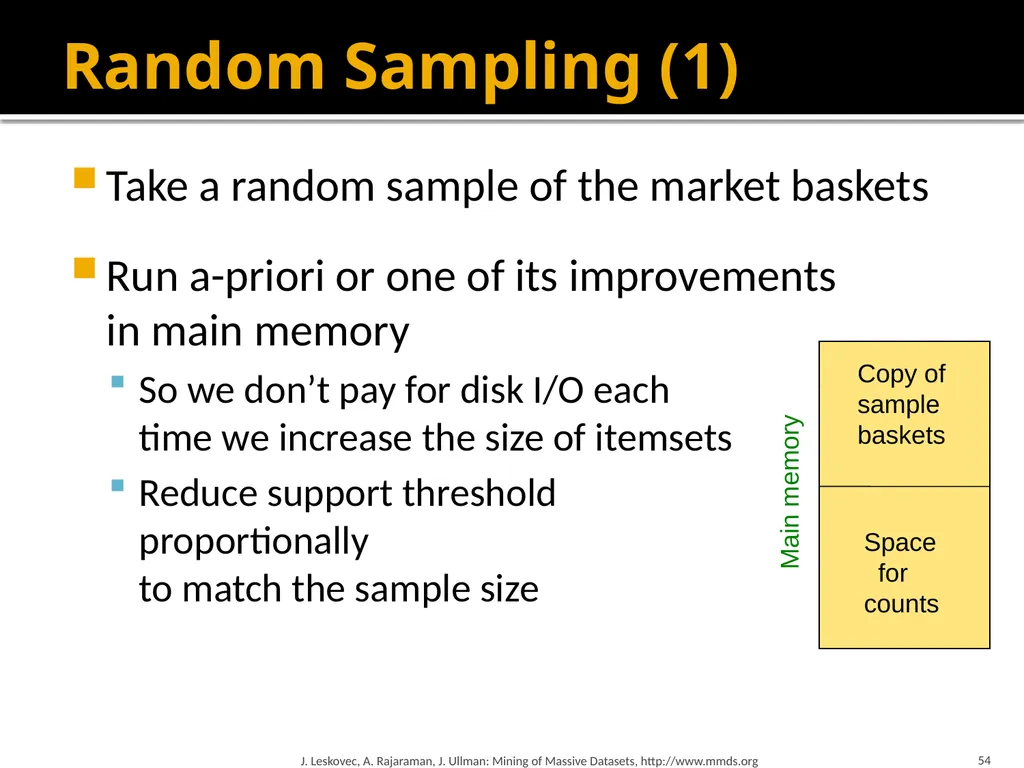
Random Sampling (1) Take a random sample of the market baskets
Run a-priori or one of its improvements in main memory
So we don’t pay for disk I/O each time we increase the size of itemsets
Reduce support threshold proportionally to match the sample size J. Leskovec, A. Rajaraman, J. Ullman: Mining of Massive Datasets, http://www.mmds.org 54 Copy of
sample
baskets Space
for
counts Main memory<br>
Run a-priori or one of its improvements in main memory
So we don’t pay for disk I/O each time we increase the size of itemsets
Reduce support threshold proportionally to match the sample size J. Leskovec, A. Rajaraman, J. Ullman: Mining of Massive Datasets, http://www.mmds.org 54 Copy of
sample
baskets Space
for
counts Main memory<br>
55
Random Sampling (2) Optionally, verify that the candidate pairs are truly frequent in the entire data set by a second pass (avoid false positives)
But you don’t catch sets frequent in the whole but not in the sample
Smaller threshold, e.g., s/125, helps catch more truly frequent itemsets
But requires more space J. Leskovec, A. Rajaraman, J. Ullman: Mining of Massive Datasets, http://www.mmds.org 55<br>
But you don’t catch sets frequent in the whole but not in the sample
Smaller threshold, e.g., s/125, helps catch more truly frequent itemsets
But requires more space J. Leskovec, A. Rajaraman, J. Ullman: Mining of Massive Datasets, http://www.mmds.org 55<br>
56
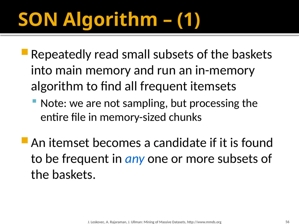
56 SON Algorithm – (1) Repeatedly read small subsets of the baskets into main memory and run an in-memory algorithm to find all frequent itemsets
Note: we are not sampling, but processing the entire file in memory-sized chunks
An itemset becomes a candidate if it is found to be frequent in any one or more subsets of the baskets. J. Leskovec, A. Rajaraman, J. Ullman: Mining of Massive Datasets, http://www.mmds.org<br>
Note: we are not sampling, but processing the entire file in memory-sized chunks
An itemset becomes a candidate if it is found to be frequent in any one or more subsets of the baskets. J. Leskovec, A. Rajaraman, J. Ullman: Mining of Massive Datasets, http://www.mmds.org<br>
57
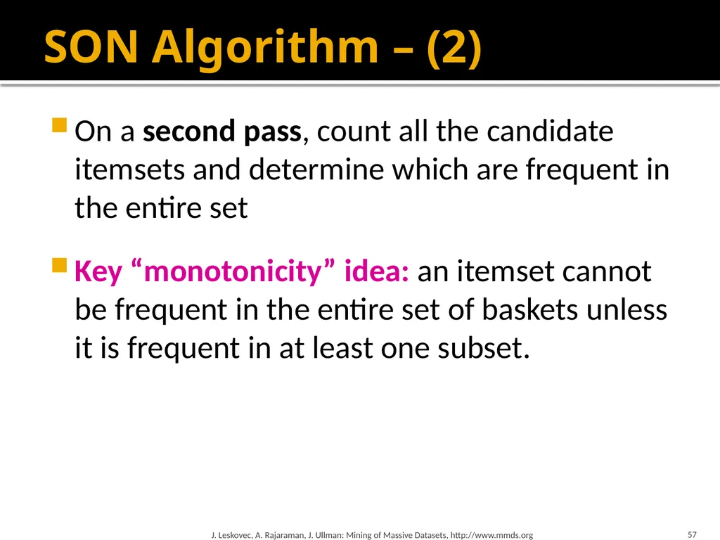
57 SON Algorithm – (2) On a second pass, count all the candidate itemsets and determine which are frequent in the entire set
Key “monotonicity” idea: an itemset cannot be frequent in the entire set of baskets unless it is frequent in at least one subset. J. Leskovec, A. Rajaraman, J. Ullman: Mining of Massive Datasets, http://www.mmds.org<br>
Key “monotonicity” idea: an itemset cannot be frequent in the entire set of baskets unless it is frequent in at least one subset. J. Leskovec, A. Rajaraman, J. Ullman: Mining of Massive Datasets, http://www.mmds.org<br>
58
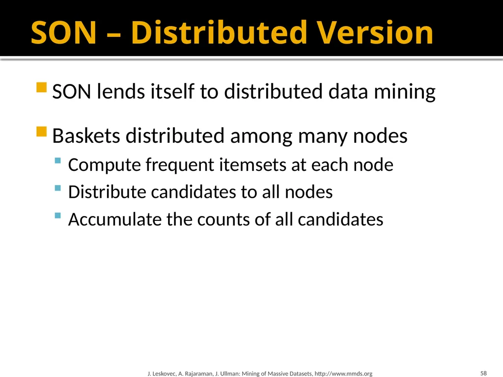
SON – Distributed Version SON lends itself to distributed data mining
Baskets distributed among many nodes
Compute frequent itemsets at each node
Distribute candidates to all nodes
Accumulate the counts of all candidates J. Leskovec, A. Rajaraman, J. Ullman: Mining of Massive Datasets, http://www.mmds.org 58<br>
Baskets distributed among many nodes
Compute frequent itemsets at each node
Distribute candidates to all nodes
Accumulate the counts of all candidates J. Leskovec, A. Rajaraman, J. Ullman: Mining of Massive Datasets, http://www.mmds.org 58<br>
59
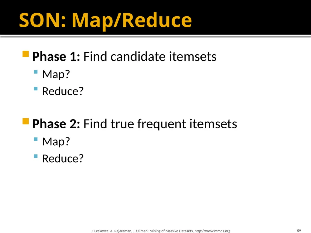
SON: Map/Reduce Phase 1: Find candidate itemsets
Map?
Reduce?
Phase 2: Find true frequent itemsets
Map?
Reduce? J. Leskovec, A. Rajaraman, J. Ullman: Mining of Massive Datasets, http://www.mmds.org 59<br>
Map?
Reduce?
Phase 2: Find true frequent itemsets
Map?
Reduce? J. Leskovec, A. Rajaraman, J. Ullman: Mining of Massive Datasets, http://www.mmds.org 59<br>