General Circulation and Chaos in Atmospheric
Description: General Circulation and Chaos in Atmospheric Predictability Waqar Younas PhD Candidate Outline General Circulation of the Atmosphere --- Atmospheric layers --- Hadley Cell --- Ferrel Cell --- Polar Cell Chaos in Atmospheric Predictability
Related Topics
Download Presentation
"General Circulation and Chaos in Atmospheric" is the property of its rightful owner. Permission is granted to download and print the materials on this website for personal, non-commercial use only, and to display it on your personal computer provided you do not modify the materials and that you retain all copyright notices contained in the materials. By downloading content from our website, you accept the terms of this agreement.
Presentation Transcript
slide1. General Circulation and Chaos in Atmospheric Predictability Waqar Younas
PhD Candidate<br>
slide2. Outline General Circulation of the Atmosphere
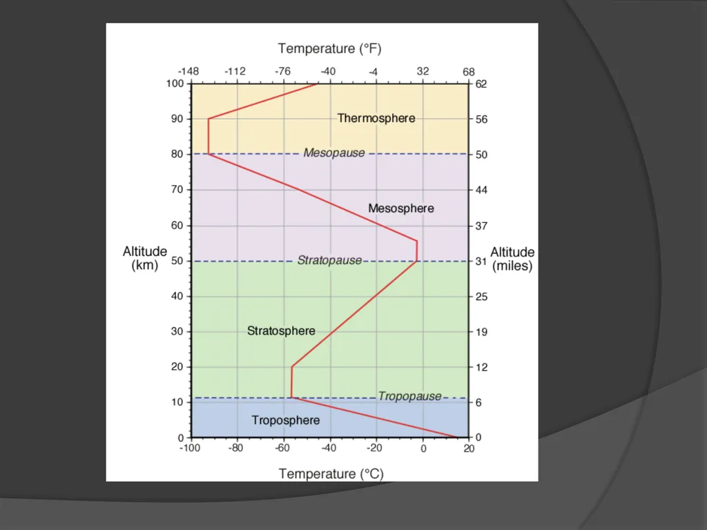
--- Atmospheric layers
--- Hadley Cell
--- Ferrel Cell
--- Polar Cell
Chaos in Atmospheric Predictability
--- Chaos
--- Predictability
--- Ensemble forecasting<br>
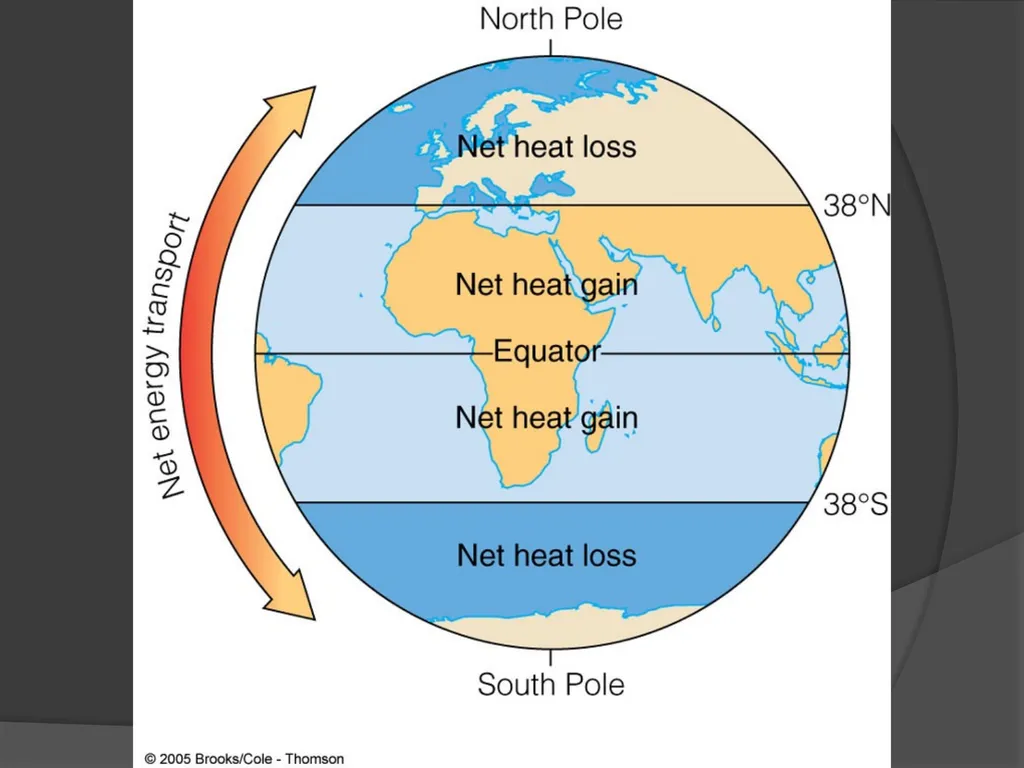
slide4. Atmospheric Circulation Powered by sunlight – uneven solar heating
About 51% of incoming energy is absorbed by Earth’s land and water
Energy absorption varies depending on the angle of approach, the sea state and the presence of ice or other covering<br>
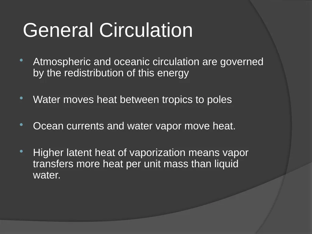
slide6. General Circulation Atmospheric and oceanic circulation are governed by the redistribution of this energy
Water moves heat between tropics to poles
Ocean currents and water vapor move heat.
Higher latent heat of vaporization means vapor transfers more heat per unit mass than liquid water.<br>
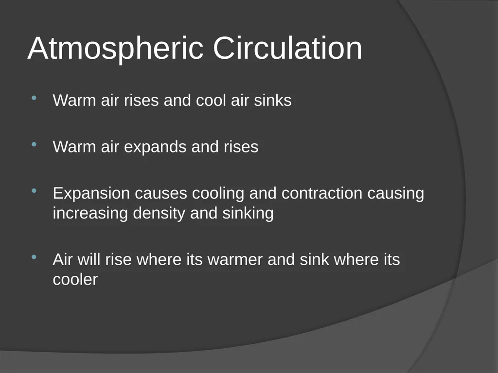
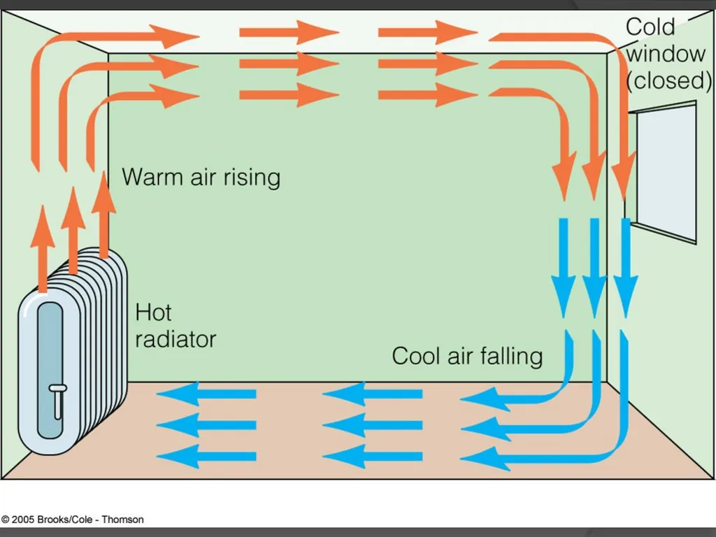
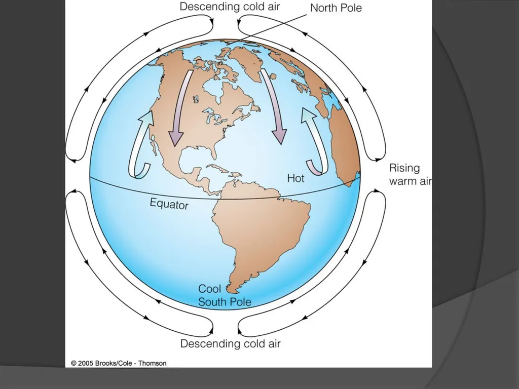
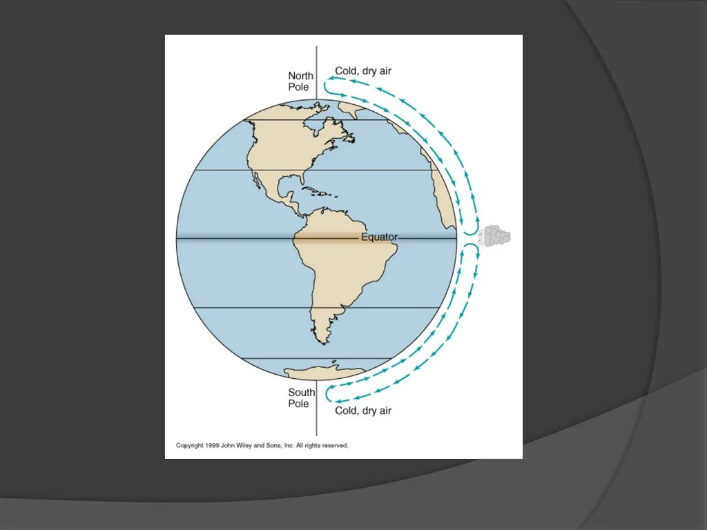
slide7. Atmospheric Circulation Warm air rises and cool air sinks
Warm air expands and rises
Expansion causes cooling and contraction causing increasing density and sinking
Air will rise where its warmer and sink where its cooler<br>
slide11. Atmospheric Circulation But, this is NOT what happens
Atmospheric circulation is governed not only by uneven solar heating but,
The Earth’s rotation
Eastward rotation of the Earth on its axis deflects moving air or water (or any object with mass).
CORIOLIS effect (1835)<br>
slide12. Coriolis Force Rotation of the Earth
Relative speeds of sphere at different latitudes
Caused by an observer’s moving frame of reference on a spinning Earth
Curve is slightly to the right of initial path in the northern hemisphere
Curve is slightly to the left of initial path in the southern hemisphere<br>
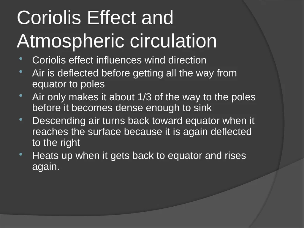
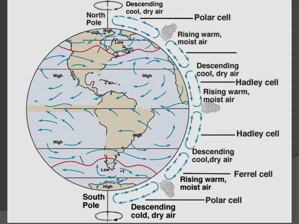
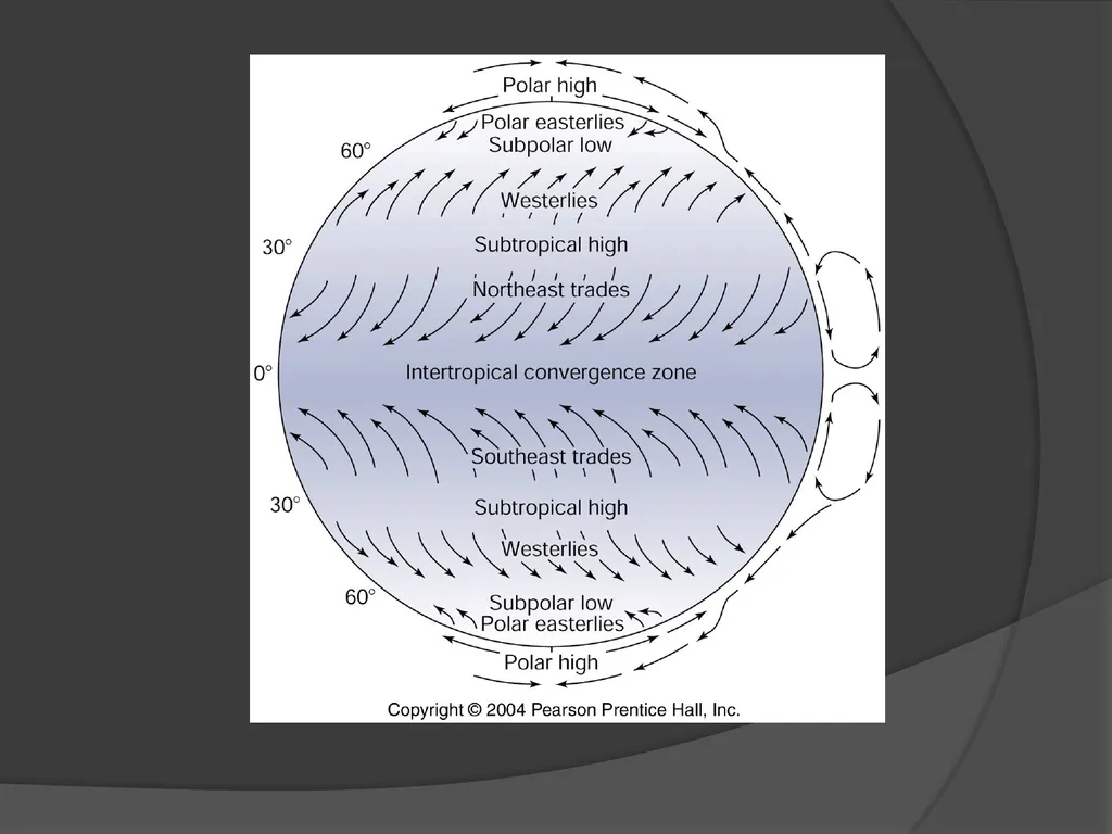
slide13. Coriolis Effect and Atmospheric circulation Coriolis effect influences wind direction
Air is deflected before getting all the way from equator to poles
Air only makes it about 1/3 of the way to the poles before it becomes dense enough to sink
Descending air turns back toward equator when it reaches the surface because it is again deflected to the right
Heats up when it gets back to equator and rises again.<br>
slide16. Chaos and Atmospheric Predictability<br>
slide17. Chaos Theory Chaos Theory Defined: a field of study in mathematics, physics, economics, and philosophy studying the behavior of dynamic systems that are highly sensitive to initial conditions.
Meteorology and Climatology<br>
slide18. Edward Lorenz “Observed” In 1961, Lorenz was using a numerical computer model to rerun a weather prediction, when, as a shortcut on a number in the sequence, he entered the decimal .506 instead of entering the full .506127 the computer would hold.
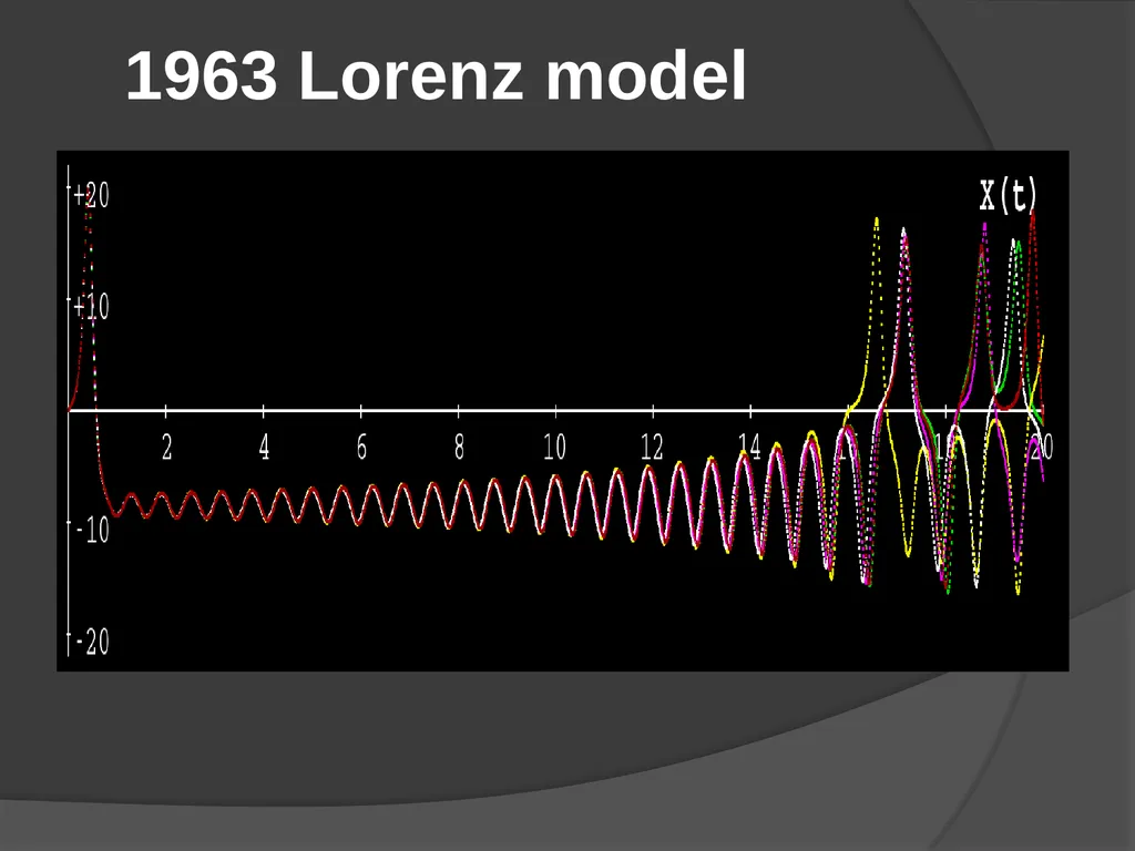
After a simulated month or so, the weather pattern diverged from the original result. A difference in the fourth decimal place was amplified in the thousands of arithmetic operations, spreading through the computation to bring a totally new outcome.
"It was possible to plug the uncertainty into an actual equation," Lorenz later recalled, "and watch the things grow, step by step."<br>
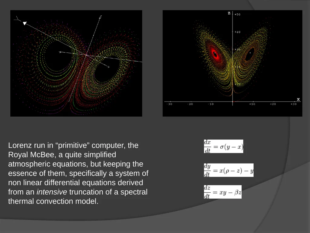
slide19. Lorenz run in “primitive” computer, the Royal McBee, a quite simplified atmospheric equations, but keeping the essence of them, specifically a system of non linear differential equations derived from an intensive truncation of a spectral thermal convection model.<br>
slide20. The truncation errors in the fourth decimal place were tiny compared with any of a hundred minor factors that might nudge the temperature or wind speed from minute to minute.
Lorenz had assumed that such variations could lead only to slightly different solutions for the equations, "recognizable as the same solution a month or a year afterwards... and it turned out to be quite different from this.“
Storms appeared or disappeared from the weather forecasts as if by chance.<br>
slide21. 1963 Lorenz model<br>
slide22. “If we claim to understand the climate system surely we should be able to predict it!”
If we cannot predict the atmosphere is this because our understanding is inadequate or are there deeper reasons?
The study of predictability concerns the systematic investigation of the extent to which it is possible to predict a system
Active area of research in weather and climate Predictability and Chaos<br>
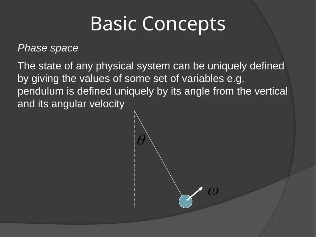
slide23. Phase space
The state of any physical system can be uniquely defined by giving the values of some set of variables e.g. pendulum is defined uniquely by its angle from the vertical and its angular velocity Basic Concepts<br>
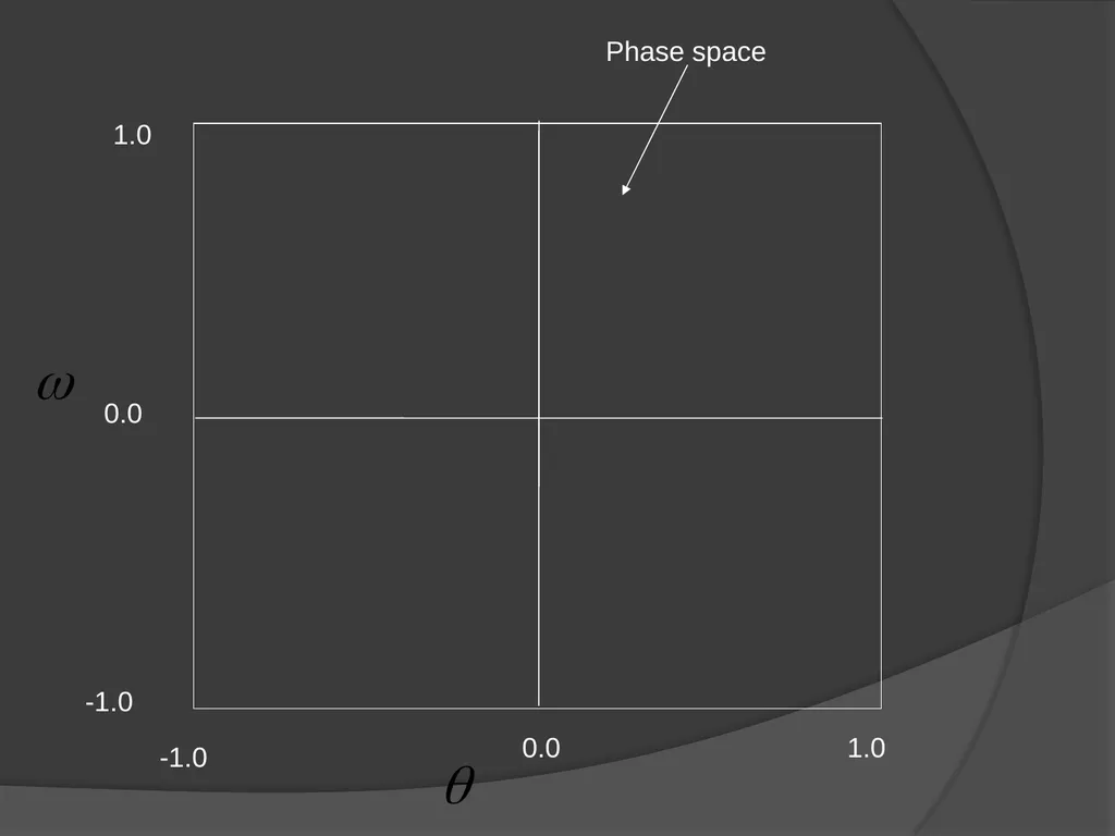
slide24. 0.0 0.0 1.0 1.0 -1.0 -1.0 Phase space<br>
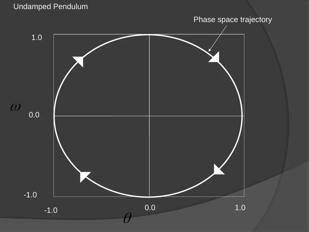
slide25. 0.0 0.0 1.0 1.0 -1.0 -1.0 Phase space trajectory Undamped Pendulum<br>
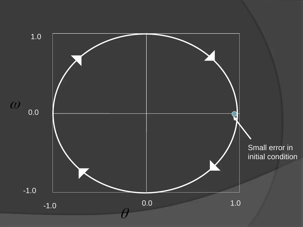
slide26. 0.0 0.0 1.0 1.0 -1.0 -1.0 Small error in initial condition<br>
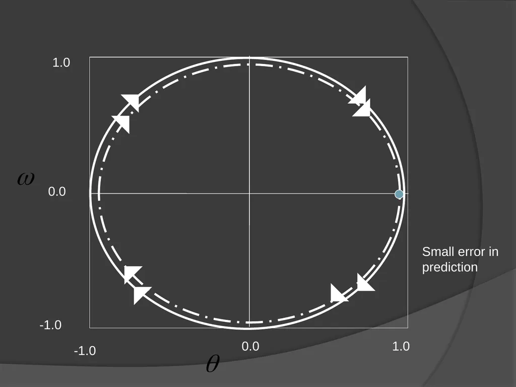
slide27. 0.0 0.0 1.0 1.0 -1.0 -1.0 Small error in prediction<br>
slide28. How do errors evolve in time? How rapidly do phase space trajectories diverge?
If diverge very slowly or not at all – then a small error in initial conditions implies a small error in the prediction of the future state – system relatively predictable
If trajectories diverge rapidly – system is unpredictable Basic Concepts<br>
slide29. Pendulum is an example of a predictable system
Two trajectories starting close together tend to stay close together
Opposite extreme – are chaotic systems – e.g. atmosphere
In these systems errors grow exponentially and thus even in a perfect model they are hard to predict far in advance
Such systems have a strong sensitivity to initial conditions<br>
slide30. Consequences of the sensitive dependence on the initial conditions
This problem has an impossible solution:
The super-computers would have to work with an infinite decimal number positions.
But both of previous points will be never possible.
On consequence, NEVER will be possible to do a PERFECT weather forecast.
Lorenz thinking way !!!<br>
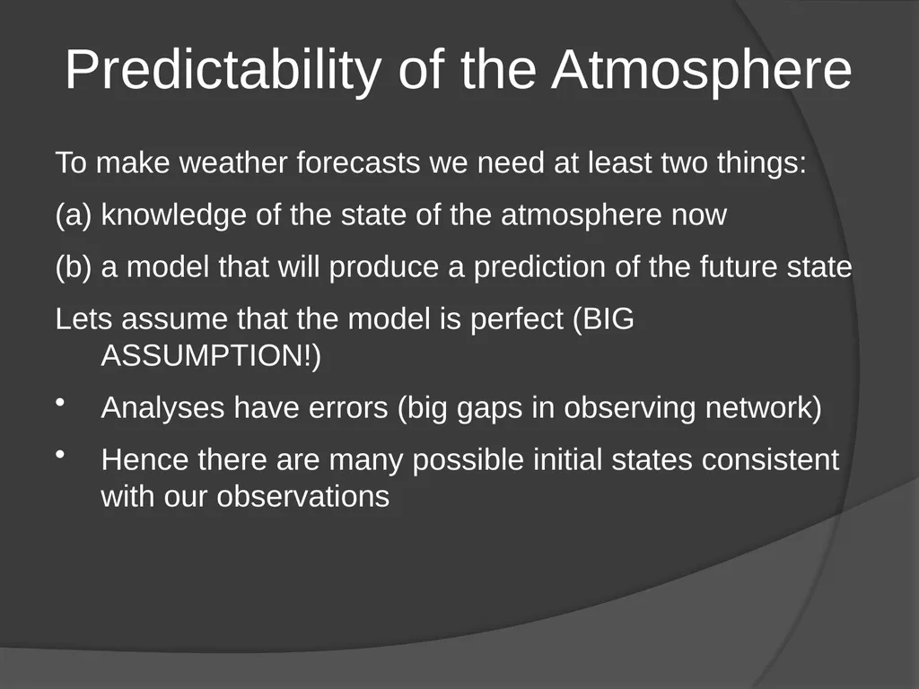
slide31. To make weather forecasts we need at least two things:
knowledge of the state of the atmosphere now
a model that will produce a prediction of the future state
Lets assume that the model is perfect (BIG ASSUMPTION!)
Analyses have errors (big gaps in observing network)
Hence there are many possible initial states consistent with our observations Predictability of the Atmosphere<br>
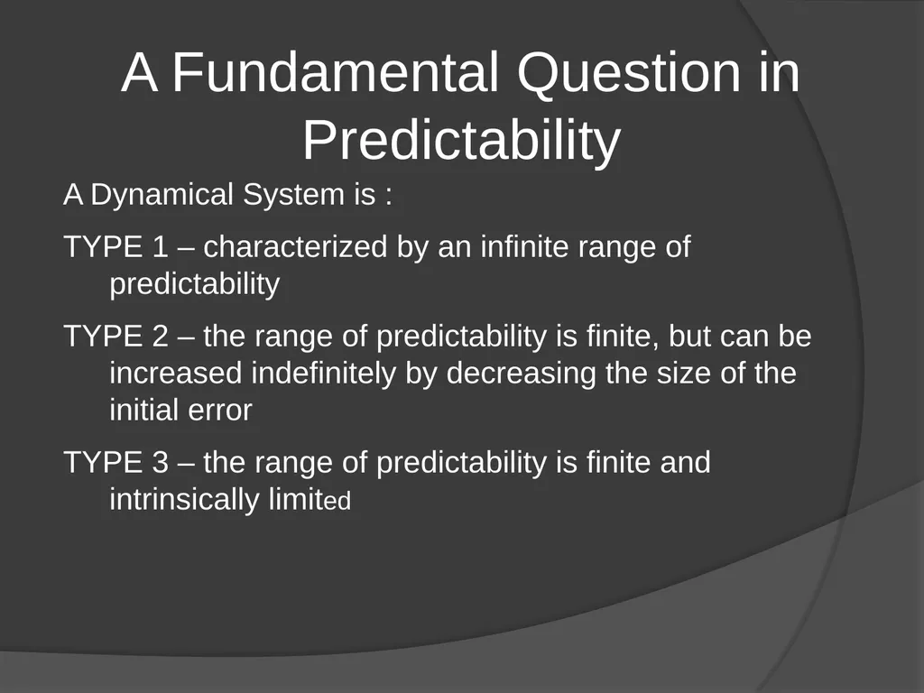
slide32. A Fundamental Question in Predictability A Dynamical System is :
TYPE 1 – characterized by an infinite range of predictability
TYPE 2 – the range of predictability is finite, but can be increased indefinitely by decreasing the size of the initial error
TYPE 3 – the range of predictability is finite and intrinsically limited<br>
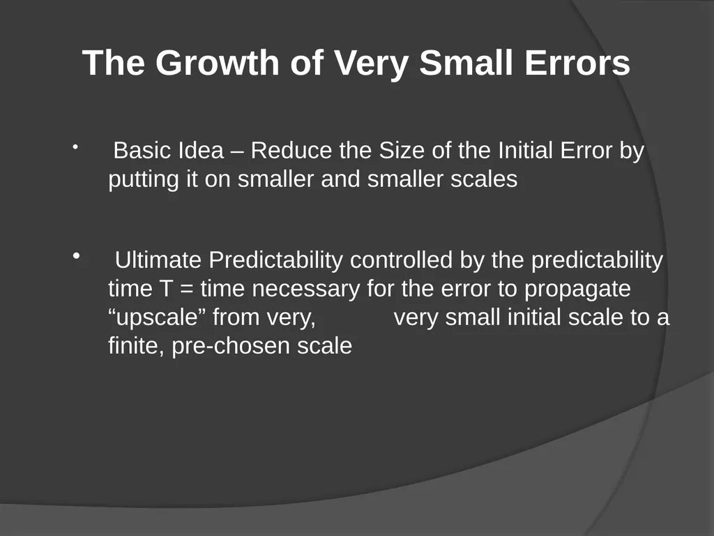
slide33. The Growth of Very Small Errors Basic Idea – Reduce the Size of the Initial Error by putting it on smaller and smaller scales
Ultimate Predictability controlled by the predictability time T = time necessary for the error to propagate “upscale” from very, very small initial scale to a finite, pre-chosen scale<br>
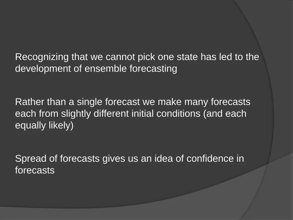
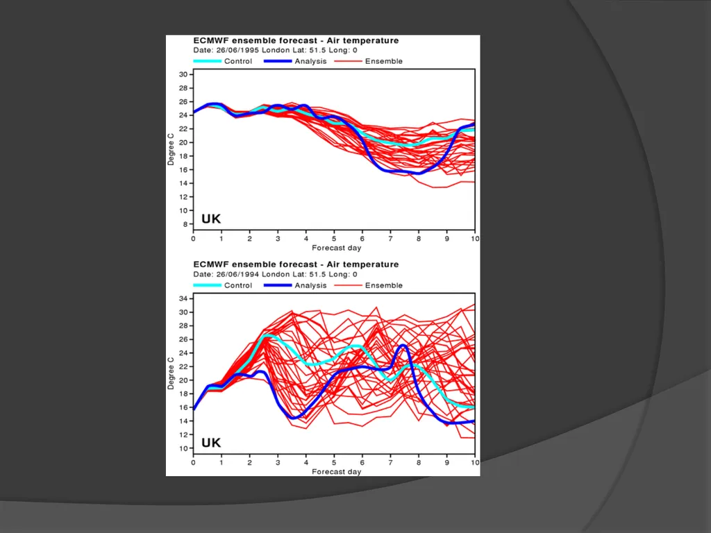
slide34. Recognizing that we cannot pick one state has led to the development of ensemble forecasting
Rather than a single forecast we make many forecasts each from slightly different initial conditions (and each equally likely)
Spread of forecasts gives us an idea of confidence in forecasts<br>
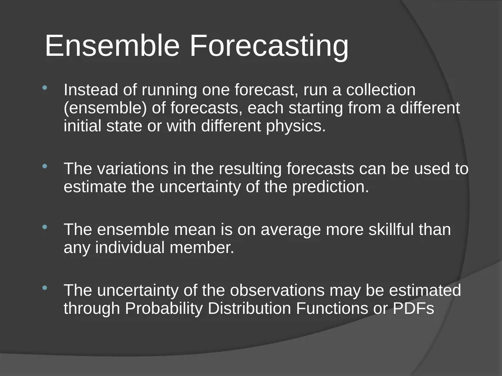
slide35. Ensemble Forecasting Instead of running one forecast, run a collection (ensemble) of forecasts, each starting from a different initial state or with different physics.
The variations in the resulting forecasts can be used to estimate the uncertainty of the prediction.
The ensemble mean is on average more skillful than any individual member.
The uncertainty of the observations may be estimated through Probability Distribution Functions or PDFs<br>
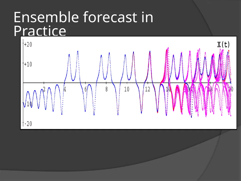
slide37. Ensemble forecast in Practice Deterministic forecast Real (observed) system evolution Ensemble<br>
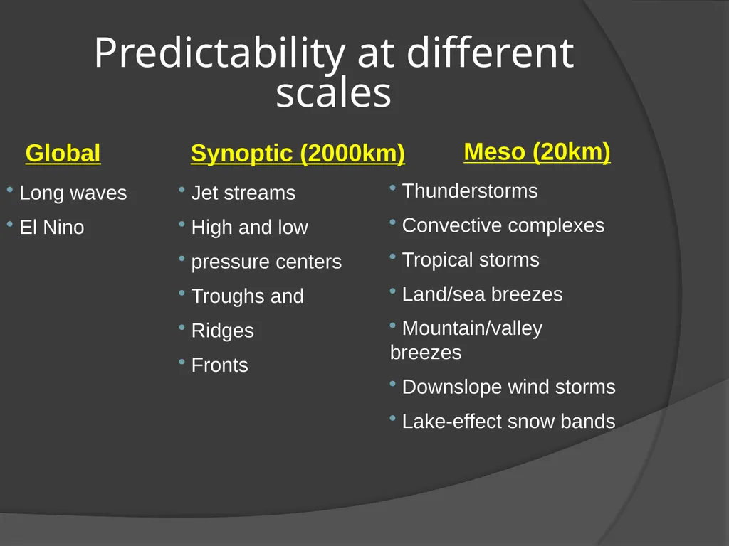
slide39. Predictability at different scales Jet streams
High and low
pressure centers
Troughs and
Ridges
Fronts Thunderstorms
Convective complexes
Tropical storms
Land/sea breezes
Mountain/valley breezes
Downslope wind storms
Lake-effect snow bands Synoptic (2000km) Meso (20km) Global Long waves
El Nino<br>
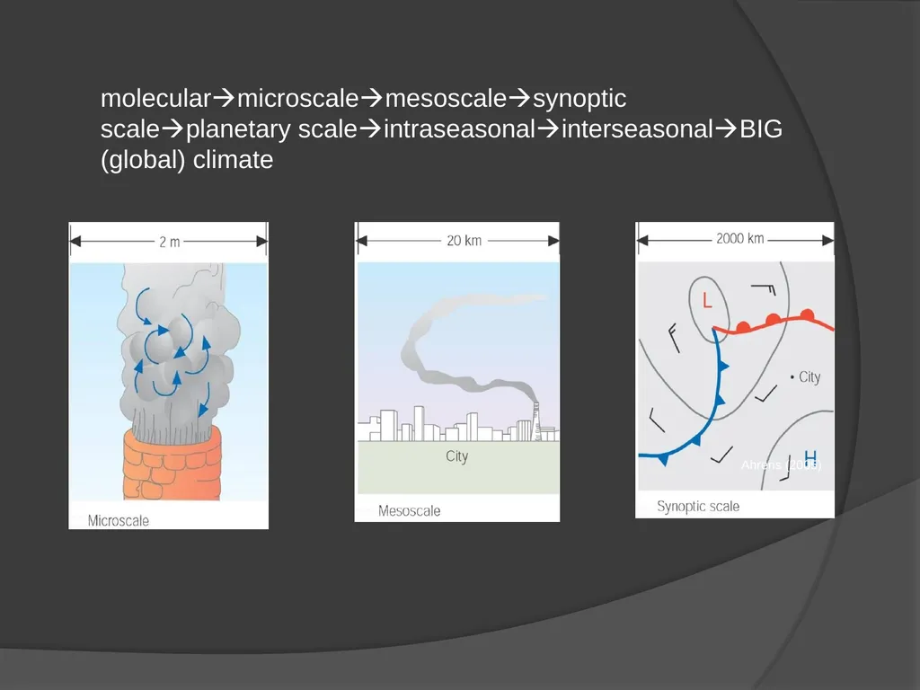
slide40. Ahrens (2005) molecularmicroscalemesoscalesynoptic scaleplanetary scaleintraseasonalinterseasonalBIG (global) climate<br>
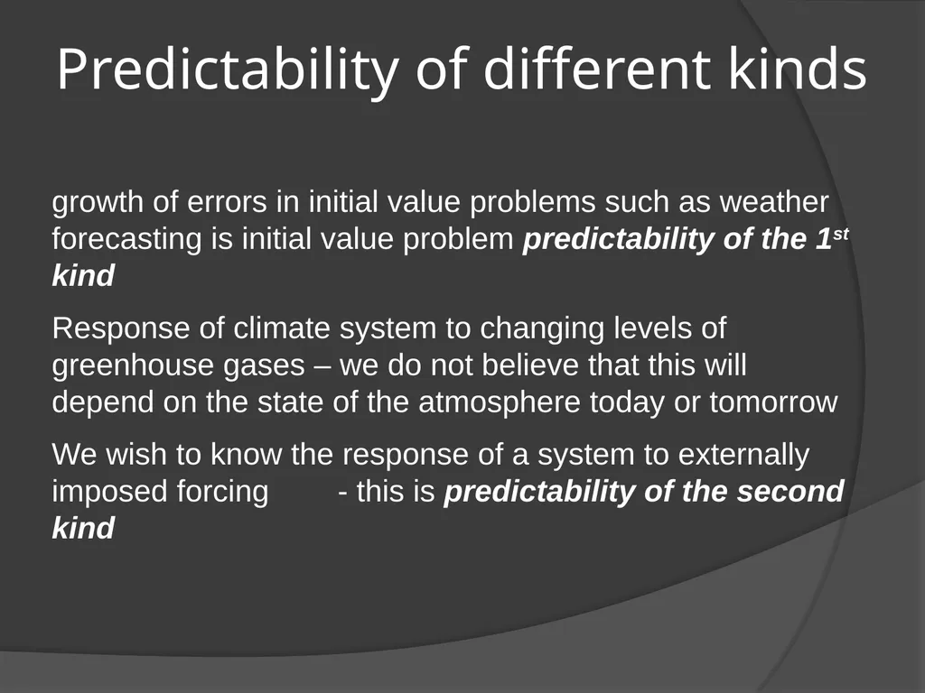
slide41. growth of errors in initial value problems such as weather forecasting is initial value problem predictability of the 1st kind
Response of climate system to changing levels of greenhouse gases – we do not believe that this will depend on the state of the atmosphere today or tomorrow
We wish to know the response of a system to externally imposed forcing - this is predictability of the second kind Predictability of different kinds<br>
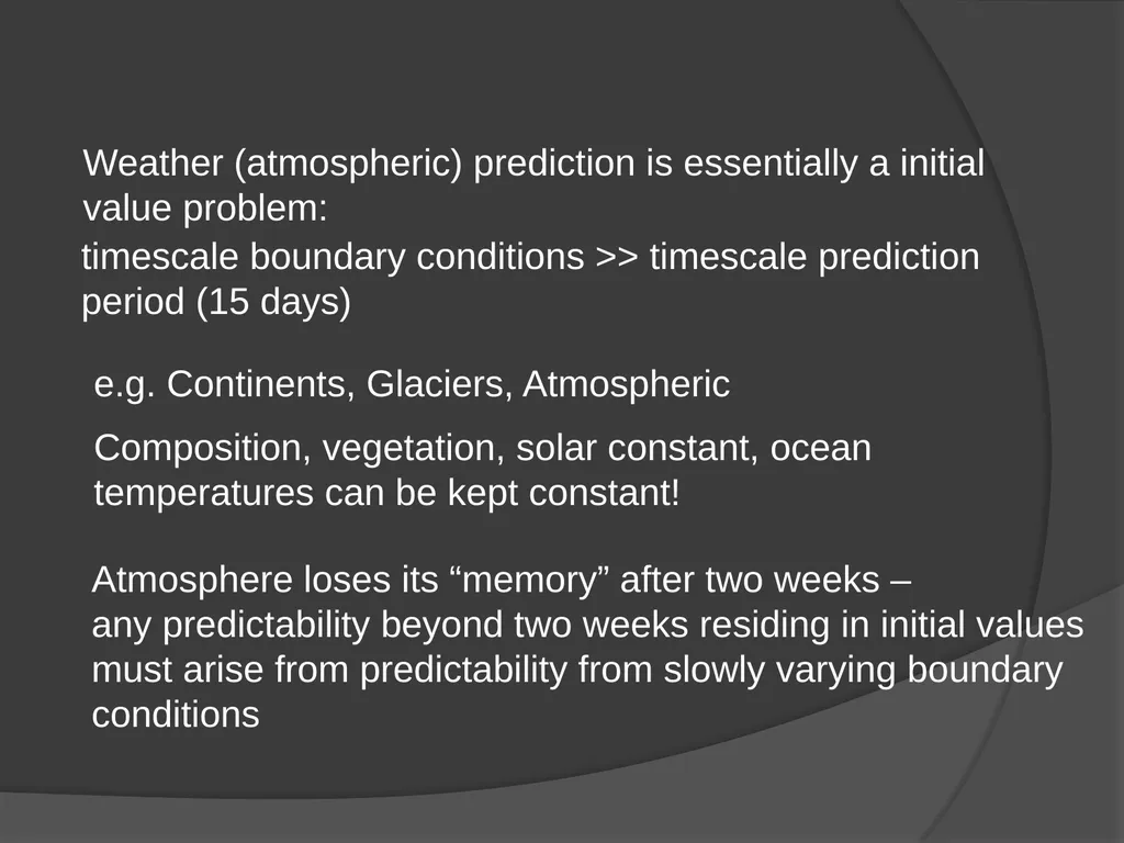
slide42. Weather (atmospheric) prediction is essentially a initial value problem: timescale boundary conditions >> timescale prediction period (15 days) e.g. Continents, Glaciers, Atmospheric
Composition, vegetation, solar constant, ocean temperatures can be kept constant! Atmosphere loses its “memory” after two weeks –
any predictability beyond two weeks residing in initial values
must arise from predictability from slowly varying boundary conditions<br>
slide43. Conclusions In predicting the atmospheric evolution, numerical prediction models are used to observe the evolution of the atmospheric states: that is, it is an information program which has most of our current knowledge about the atmosphere.
It will NEVER be possible to do a PERFECT FORECAST of the future state of the atmosphere.
But it is possible to estimate the predictability of the future atmospheric states and limit their uncertainty through probabilistic forecasts drawn from ensembles.<br>

slide44. Thank You!<br>
PhD Candidate<br>
slide2. Outline General Circulation of the Atmosphere
--- Atmospheric layers
--- Hadley Cell
--- Ferrel Cell
--- Polar Cell
Chaos in Atmospheric Predictability
--- Chaos
--- Predictability
--- Ensemble forecasting<br>
slide4. Atmospheric Circulation Powered by sunlight – uneven solar heating
About 51% of incoming energy is absorbed by Earth’s land and water
Energy absorption varies depending on the angle of approach, the sea state and the presence of ice or other covering<br>
slide6. General Circulation Atmospheric and oceanic circulation are governed by the redistribution of this energy
Water moves heat between tropics to poles
Ocean currents and water vapor move heat.
Higher latent heat of vaporization means vapor transfers more heat per unit mass than liquid water.<br>
slide7. Atmospheric Circulation Warm air rises and cool air sinks
Warm air expands and rises
Expansion causes cooling and contraction causing increasing density and sinking
Air will rise where its warmer and sink where its cooler<br>
slide11. Atmospheric Circulation But, this is NOT what happens
Atmospheric circulation is governed not only by uneven solar heating but,
The Earth’s rotation
Eastward rotation of the Earth on its axis deflects moving air or water (or any object with mass).
CORIOLIS effect (1835)<br>
slide12. Coriolis Force Rotation of the Earth
Relative speeds of sphere at different latitudes
Caused by an observer’s moving frame of reference on a spinning Earth
Curve is slightly to the right of initial path in the northern hemisphere
Curve is slightly to the left of initial path in the southern hemisphere<br>
slide13. Coriolis Effect and Atmospheric circulation Coriolis effect influences wind direction
Air is deflected before getting all the way from equator to poles
Air only makes it about 1/3 of the way to the poles before it becomes dense enough to sink
Descending air turns back toward equator when it reaches the surface because it is again deflected to the right
Heats up when it gets back to equator and rises again.<br>
slide16. Chaos and Atmospheric Predictability<br>
slide17. Chaos Theory Chaos Theory Defined: a field of study in mathematics, physics, economics, and philosophy studying the behavior of dynamic systems that are highly sensitive to initial conditions.
Meteorology and Climatology<br>
slide18. Edward Lorenz “Observed” In 1961, Lorenz was using a numerical computer model to rerun a weather prediction, when, as a shortcut on a number in the sequence, he entered the decimal .506 instead of entering the full .506127 the computer would hold.
After a simulated month or so, the weather pattern diverged from the original result. A difference in the fourth decimal place was amplified in the thousands of arithmetic operations, spreading through the computation to bring a totally new outcome.
"It was possible to plug the uncertainty into an actual equation," Lorenz later recalled, "and watch the things grow, step by step."<br>
slide19. Lorenz run in “primitive” computer, the Royal McBee, a quite simplified atmospheric equations, but keeping the essence of them, specifically a system of non linear differential equations derived from an intensive truncation of a spectral thermal convection model.<br>
slide20. The truncation errors in the fourth decimal place were tiny compared with any of a hundred minor factors that might nudge the temperature or wind speed from minute to minute.
Lorenz had assumed that such variations could lead only to slightly different solutions for the equations, "recognizable as the same solution a month or a year afterwards... and it turned out to be quite different from this.“
Storms appeared or disappeared from the weather forecasts as if by chance.<br>
slide21. 1963 Lorenz model<br>
slide22. “If we claim to understand the climate system surely we should be able to predict it!”
If we cannot predict the atmosphere is this because our understanding is inadequate or are there deeper reasons?
The study of predictability concerns the systematic investigation of the extent to which it is possible to predict a system
Active area of research in weather and climate Predictability and Chaos<br>
slide23. Phase space
The state of any physical system can be uniquely defined by giving the values of some set of variables e.g. pendulum is defined uniquely by its angle from the vertical and its angular velocity Basic Concepts<br>
slide24. 0.0 0.0 1.0 1.0 -1.0 -1.0 Phase space<br>
slide25. 0.0 0.0 1.0 1.0 -1.0 -1.0 Phase space trajectory Undamped Pendulum<br>
slide26. 0.0 0.0 1.0 1.0 -1.0 -1.0 Small error in initial condition<br>
slide27. 0.0 0.0 1.0 1.0 -1.0 -1.0 Small error in prediction<br>
slide28. How do errors evolve in time? How rapidly do phase space trajectories diverge?
If diverge very slowly or not at all – then a small error in initial conditions implies a small error in the prediction of the future state – system relatively predictable
If trajectories diverge rapidly – system is unpredictable Basic Concepts<br>
slide29. Pendulum is an example of a predictable system
Two trajectories starting close together tend to stay close together
Opposite extreme – are chaotic systems – e.g. atmosphere
In these systems errors grow exponentially and thus even in a perfect model they are hard to predict far in advance
Such systems have a strong sensitivity to initial conditions<br>
slide30. Consequences of the sensitive dependence on the initial conditions
This problem has an impossible solution:
The super-computers would have to work with an infinite decimal number positions.
But both of previous points will be never possible.
On consequence, NEVER will be possible to do a PERFECT weather forecast.
Lorenz thinking way !!!<br>
slide31. To make weather forecasts we need at least two things:
knowledge of the state of the atmosphere now
a model that will produce a prediction of the future state
Lets assume that the model is perfect (BIG ASSUMPTION!)
Analyses have errors (big gaps in observing network)
Hence there are many possible initial states consistent with our observations Predictability of the Atmosphere<br>
slide32. A Fundamental Question in Predictability A Dynamical System is :
TYPE 1 – characterized by an infinite range of predictability
TYPE 2 – the range of predictability is finite, but can be increased indefinitely by decreasing the size of the initial error
TYPE 3 – the range of predictability is finite and intrinsically limited<br>
slide33. The Growth of Very Small Errors Basic Idea – Reduce the Size of the Initial Error by putting it on smaller and smaller scales
Ultimate Predictability controlled by the predictability time T = time necessary for the error to propagate “upscale” from very, very small initial scale to a finite, pre-chosen scale<br>
slide34. Recognizing that we cannot pick one state has led to the development of ensemble forecasting
Rather than a single forecast we make many forecasts each from slightly different initial conditions (and each equally likely)
Spread of forecasts gives us an idea of confidence in forecasts<br>
slide35. Ensemble Forecasting Instead of running one forecast, run a collection (ensemble) of forecasts, each starting from a different initial state or with different physics.
The variations in the resulting forecasts can be used to estimate the uncertainty of the prediction.
The ensemble mean is on average more skillful than any individual member.
The uncertainty of the observations may be estimated through Probability Distribution Functions or PDFs<br>
slide37. Ensemble forecast in Practice Deterministic forecast Real (observed) system evolution Ensemble<br>
slide39. Predictability at different scales Jet streams
High and low
pressure centers
Troughs and
Ridges
Fronts Thunderstorms
Convective complexes
Tropical storms
Land/sea breezes
Mountain/valley breezes
Downslope wind storms
Lake-effect snow bands Synoptic (2000km) Meso (20km) Global Long waves
El Nino<br>
slide40. Ahrens (2005) molecularmicroscalemesoscalesynoptic scaleplanetary scaleintraseasonalinterseasonalBIG (global) climate<br>
slide41. growth of errors in initial value problems such as weather forecasting is initial value problem predictability of the 1st kind
Response of climate system to changing levels of greenhouse gases – we do not believe that this will depend on the state of the atmosphere today or tomorrow
We wish to know the response of a system to externally imposed forcing - this is predictability of the second kind Predictability of different kinds<br>
slide42. Weather (atmospheric) prediction is essentially a initial value problem: timescale boundary conditions >> timescale prediction period (15 days) e.g. Continents, Glaciers, Atmospheric
Composition, vegetation, solar constant, ocean temperatures can be kept constant! Atmosphere loses its “memory” after two weeks –
any predictability beyond two weeks residing in initial values
must arise from predictability from slowly varying boundary conditions<br>
slide43. Conclusions In predicting the atmospheric evolution, numerical prediction models are used to observe the evolution of the atmospheric states: that is, it is an information program which has most of our current knowledge about the atmosphere.
It will NEVER be possible to do a PERFECT FORECAST of the future state of the atmosphere.
But it is possible to estimate the predictability of the future atmospheric states and limit their uncertainty through probabilistic forecasts drawn from ensembles.<br>
slide44. Thank You!<br>