
Graph Guessing Games & non-Shannon Information
SN
Published · 43 slides · 0 views
1 / 1
Description
Graph Guessing Games non-Shannon Information Inequalities First workshop on Entropy and Information Inequalities 17 April 2013 Søren Riis Queen Mary University of London Overview Digraph Guessing Games Graph Entropy (causal networks)
Related Topics
Share
Embed code
Download this presentation From Below
"Graph Guessing Games & non-Shannon Information" is the property of its rightful owner. Permission is granted to download and print the materials on this website for personal, non-commercial use only, and to display it on your personal computer provided you do not modify the materials and that you retain all copyright notices contained in the materials. By downloading content from our website, you accept the terms of this agreement.
Presentation Transcript
01
Graph Guessing Games &
non-Shannon Information Inequalities First workshop on Entropy and Information Inequalities
17 April 2013
Søren Riis
Queen Mary University of London<br>
17 April 2013
Søren Riis
Queen Mary University of London<br>
02
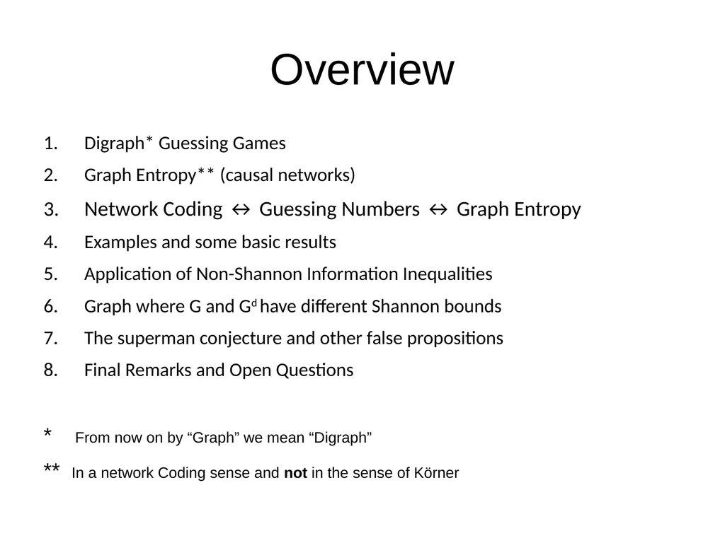
Overview Digraph* Guessing Games
Graph Entropy** (causal networks)
Network Coding ↔ Guessing Numbers ↔ Graph Entropy
Examples and some basic results
Application of Non-Shannon Information Inequalities
Graph where G and Gd have different Shannon bounds
The superman conjecture and other false propositions
Final Remarks and Open Questions
* From now on by “Graph” we mean “Digraph”
** In a network Coding sense and not in the sense of Körner<br>
Graph Entropy** (causal networks)
Network Coding ↔ Guessing Numbers ↔ Graph Entropy
Examples and some basic results
Application of Non-Shannon Information Inequalities
Graph where G and Gd have different Shannon bounds
The superman conjecture and other false propositions
Final Remarks and Open Questions
* From now on by “Graph” we mean “Digraph”
** In a network Coding sense and not in the sense of Körner<br>
03
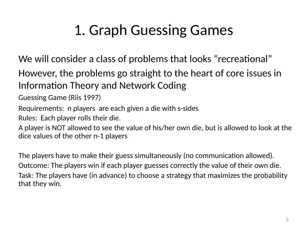
3 1. Graph Guessing Games We will consider a class of problems that looks “recreational”
However, the problems go straight to the heart of core issues in Information Theory and Network Coding
Guessing Game (Riis 1997)
Requirements: n players are each given a die with s-sides
Rules: Each player rolls their die.
A player is NOT allowed to see the value of his/her own die, but is allowed to look at the dice values of the other n-1 players
The players have to make their guess simultaneously (no communication allowed).
Outcome: The players win if each player guesses correctly the value of their own die.
Task: The players have (in advance) to choose a strategy that maximizes the probability that they win.<br>
However, the problems go straight to the heart of core issues in Information Theory and Network Coding
Guessing Game (Riis 1997)
Requirements: n players are each given a die with s-sides
Rules: Each player rolls their die.
A player is NOT allowed to see the value of his/her own die, but is allowed to look at the dice values of the other n-1 players
The players have to make their guess simultaneously (no communication allowed).
Outcome: The players win if each player guesses correctly the value of their own die.
Task: The players have (in advance) to choose a strategy that maximizes the probability that they win.<br>
04
1. Graph Guessing Games
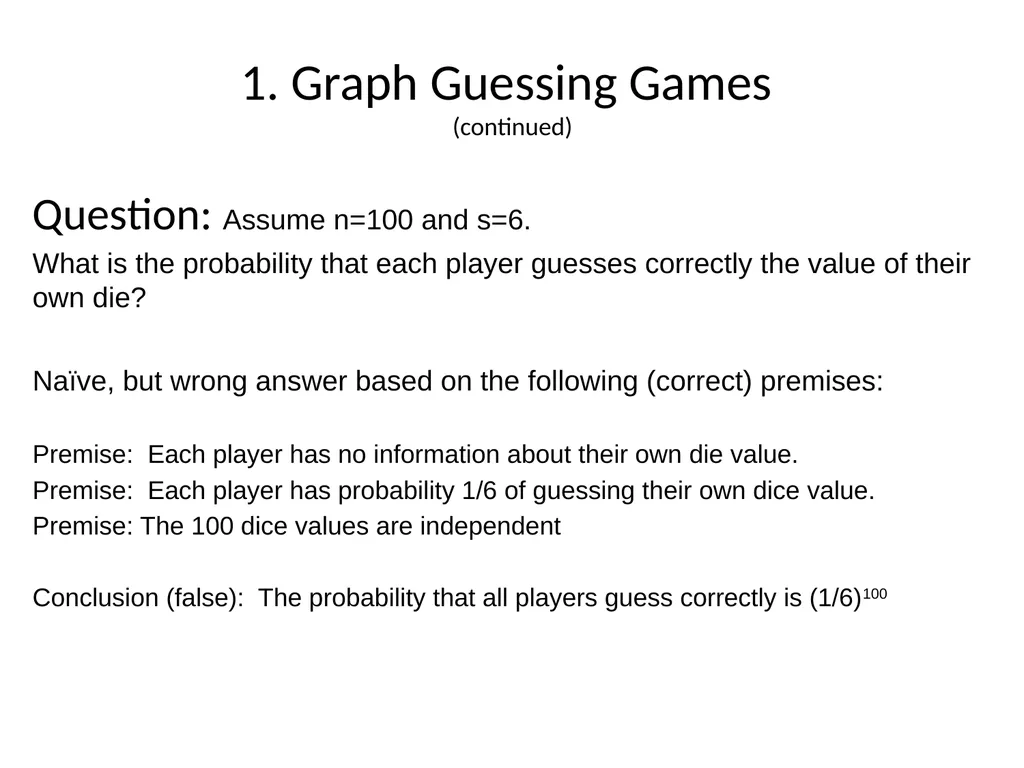
(continued) Question: Assume n=100 and s=6.
What is the probability that each player guesses correctly the value of their own die?
Naïve, but wrong answer based on the following (correct) premises:
Premise: Each player has no information about their own die value.
Premise: Each player has probability 1/6 of guessing their own dice value.
Premise: The 100 dice values are independent
Conclusion (false): The probability that all players guess correctly is (1/6)100<br>
What is the probability that each player guesses correctly the value of their own die?
Naïve, but wrong answer based on the following (correct) premises:
Premise: Each player has no information about their own die value.
Premise: Each player has probability 1/6 of guessing their own dice value.
Premise: The 100 dice values are independent
Conclusion (false): The probability that all players guess correctly is (1/6)100<br>
05
5 Graph Guessing Games
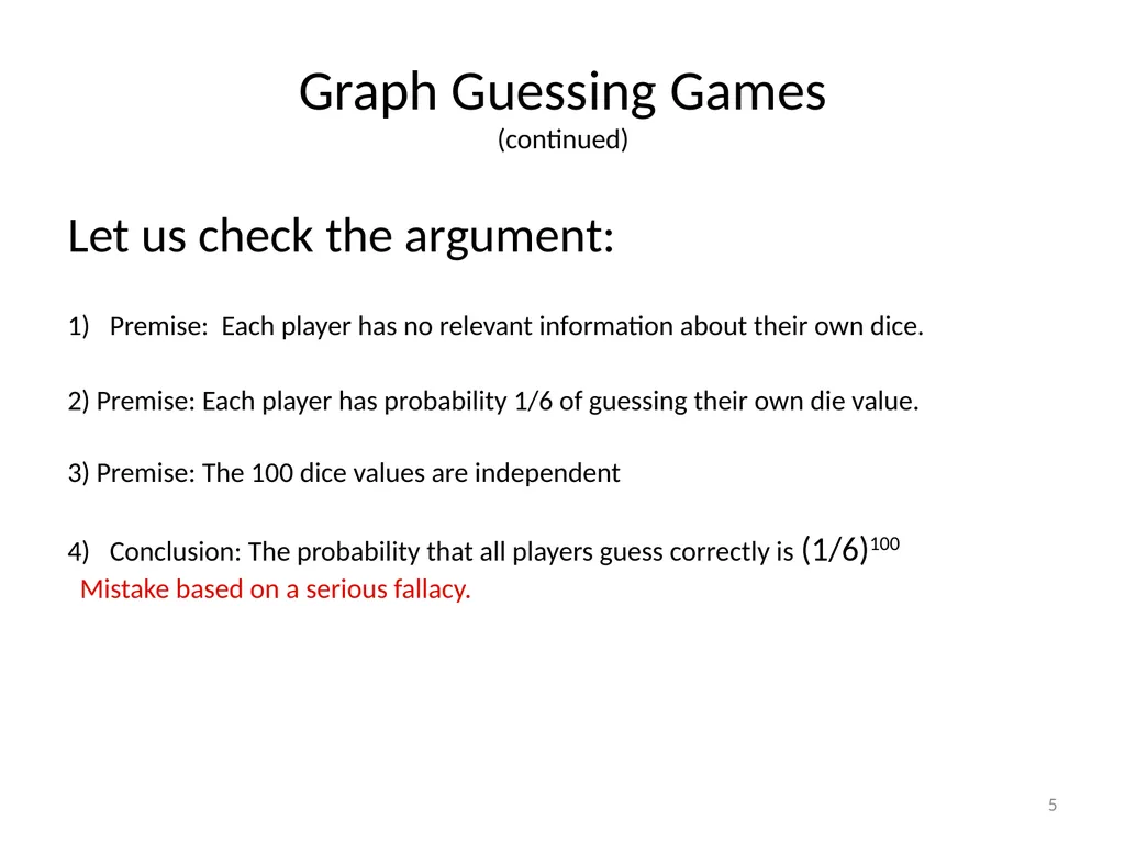
(continued) Let us check the argument:
Premise: Each player has no relevant information about their own dice.
2) Premise: Each player has probability 1/6 of guessing their own die value.
3) Premise: The 100 dice values are independent
Conclusion: The probability that all players guess correctly is (1/6)100
Mistake based on a serious fallacy.<br>
Premise: Each player has no relevant information about their own dice.
2) Premise: Each player has probability 1/6 of guessing their own die value.
3) Premise: The 100 dice values are independent
Conclusion: The probability that all players guess correctly is (1/6)100
Mistake based on a serious fallacy.<br>
06
Graph Guessing Games
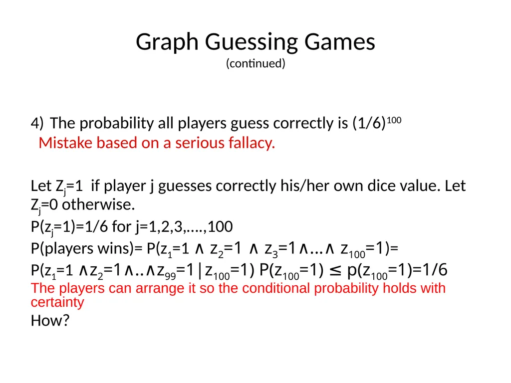
(continued) The probability all players guess correctly is (1/6)100
Mistake based on a serious fallacy.
Let Zj=1 if player j guesses correctly his/her own dice value. Let Zj=0 otherwise.
P(zj=1)=1/6 for j=1,2,3,….,100
P(players wins)= P(z1=1 ∧ z2=1 ∧ z3=1∧...∧ z100=1)=
P(z1=1 ∧z2=1∧..∧z99=1|z100=1) P(z100=1) ≤ p(z100=1)=1/6
The players can arrange it so the conditional probability holds with certainty
How?<br>
Mistake based on a serious fallacy.
Let Zj=1 if player j guesses correctly his/her own dice value. Let Zj=0 otherwise.
P(zj=1)=1/6 for j=1,2,3,….,100
P(players wins)= P(z1=1 ∧ z2=1 ∧ z3=1∧...∧ z100=1)=
P(z1=1 ∧z2=1∧..∧z99=1|z100=1) P(z100=1) ≤ p(z100=1)=1/6
The players can arrange it so the conditional probability holds with certainty
How?<br>
07
7 Graph Guessing Games
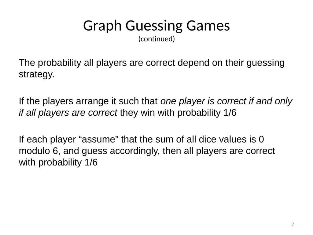
(continued) The probability all players are correct depend on their guessing strategy.
If the players arrange it such that one player is correct if and only if all players are correct they win with probability 1/6
If each player “assume” that the sum of all dice values is 0 modulo 6, and guess accordingly, then all players are correct with probability 1/6<br>
If the players arrange it such that one player is correct if and only if all players are correct they win with probability 1/6
If each player “assume” that the sum of all dice values is 0 modulo 6, and guess accordingly, then all players are correct with probability 1/6<br>
08
Graph Guessing Games
(continued) The uncoordinated guessing strategy succeeds with probability (1/s)n
The optimal guessing strategy succeeds with probability 1/s
Thus by cooperating the players can achieve a probability that is s(n-1) times more likely of succeeding than a uncoordinated guessing strategy.
The power n-1 in the factor s(n-1) plays an important role in our theory.<br>
The optimal guessing strategy succeeds with probability 1/s
Thus by cooperating the players can achieve a probability that is s(n-1) times more likely of succeeding than a uncoordinated guessing strategy.
The power n-1 in the factor s(n-1) plays an important role in our theory.<br>
09
9 Graph Guessing Games
(continued) Graph Guessing Game (Riis 2005)
Requirements: n players are each given a die with s-sides
Rules: Each player rolls their die.
Each player is sitting in a node in a given graph.
A player has only access to the dice values of their direct predecessors.
The players have to make their guess simultaneously
Outcome: The players win if each player guesses correctly the value of their own die.
Task: The players have (in advance) to choose a strategy that maximizes the probability that they win.<br>
Requirements: n players are each given a die with s-sides
Rules: Each player rolls their die.
Each player is sitting in a node in a given graph.
A player has only access to the dice values of their direct predecessors.
The players have to make their guess simultaneously
Outcome: The players win if each player guesses correctly the value of their own die.
Task: The players have (in advance) to choose a strategy that maximizes the probability that they win.<br>
10
10 Graph Guessing Games
(continued) Definition:
The guessing number of a graph G (or strategy)
is α if the players can succeed with a probability that is sα times higher than the probability of success when using uncoordinated random guessing.
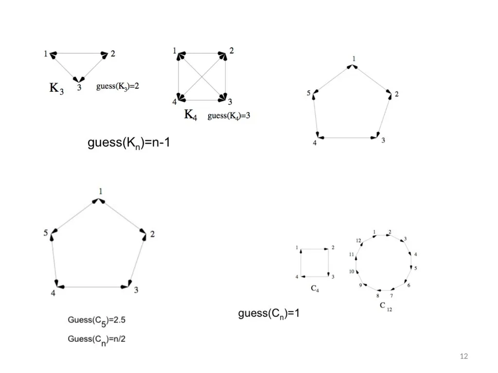
The complete graph Knwith bi-directed edges, corresponds to the guessing game we already considered.
Proposition:
The guessing number guess(Kn) of Kn is n-1 because we can do s(n-1) times better than uncoordinated random guessing.
Notice that the guessing number of Kn does not depend on the size s of the “alphabet”<br>
The guessing number of a graph G (or strategy)
is α if the players can succeed with a probability that is sα times higher than the probability of success when using uncoordinated random guessing.
The complete graph Knwith bi-directed edges, corresponds to the guessing game we already considered.
Proposition:
The guessing number guess(Kn) of Kn is n-1 because we can do s(n-1) times better than uncoordinated random guessing.
Notice that the guessing number of Kn does not depend on the size s of the “alphabet”<br>
11
11 Graph Guessing Games
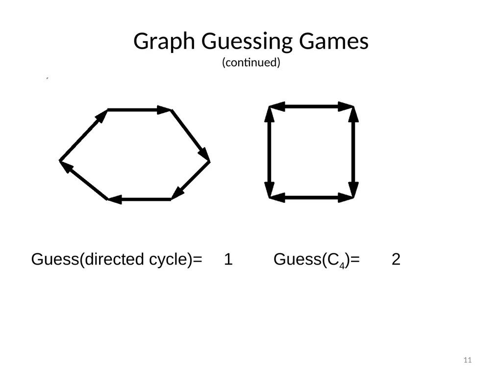
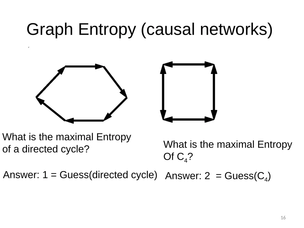
(continued) Guess(directed cycle)= 1 Guess(C4)= 2<br>
12
12<br>
13
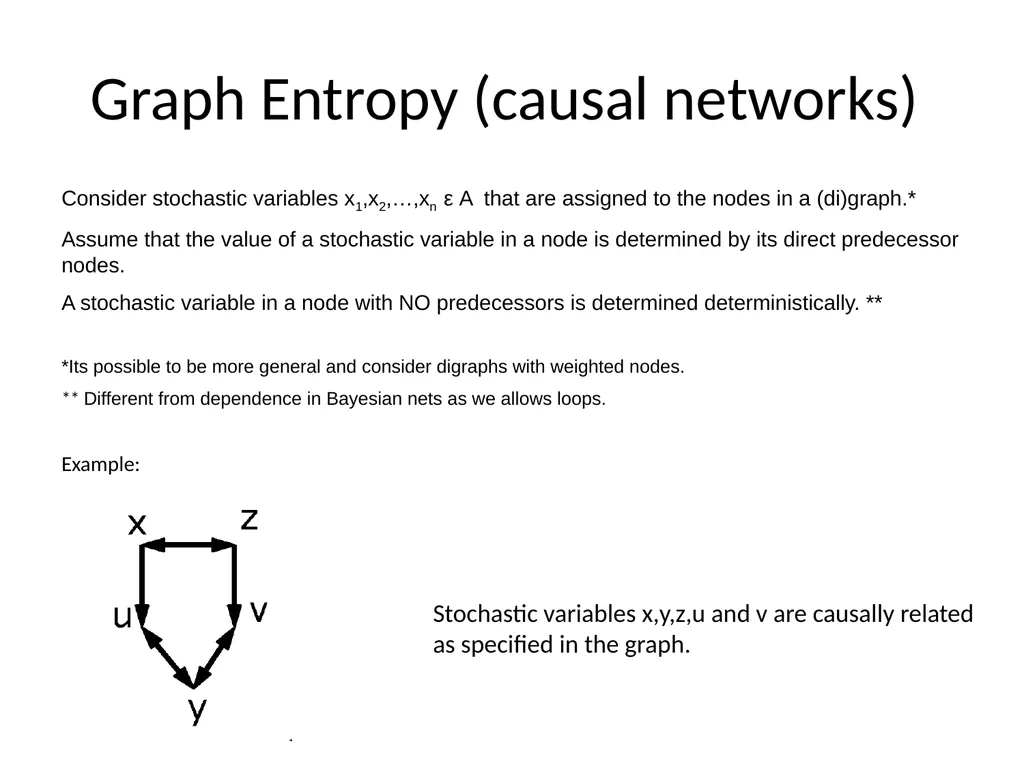
Graph Entropy (causal networks) Consider stochastic variables x1,x2,…,xn ε A that are assigned to the nodes in a (di)graph.*
Assume that the value of a stochastic variable in a node is determined by its direct predecessor nodes.
A stochastic variable in a node with NO predecessors is determined deterministically. **
*Its possible to be more general and consider digraphs with weighted nodes.
** Different from dependence in Bayesian nets as we allows loops.
Example: Stochastic variables x,y,z,u and v are causally related
as specified in the graph.<br>
Assume that the value of a stochastic variable in a node is determined by its direct predecessor nodes.
A stochastic variable in a node with NO predecessors is determined deterministically. **
*Its possible to be more general and consider digraphs with weighted nodes.
** Different from dependence in Bayesian nets as we allows loops.
Example: Stochastic variables x,y,z,u and v are causally related
as specified in the graph.<br>
14
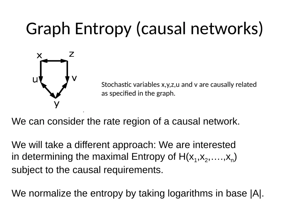
Graph Entropy (causal networks) Stochastic variables x,y,z,u and v are causally related
as specified in the graph. We can consider the rate region of a causal network.
We will take a different approach: We are interested
in determining the maximal Entropy of H(x1,x2,….,xn)
subject to the causal requirements.
We normalize the entropy by taking logarithms in base |A|.<br>
as specified in the graph. We can consider the rate region of a causal network.
We will take a different approach: We are interested
in determining the maximal Entropy of H(x1,x2,….,xn)
subject to the causal requirements.
We normalize the entropy by taking logarithms in base |A|.<br>
15
Graph Entropy (causal networks) We will take a different approach: We are interested
In determining the maximal Entropy of H(x1,x2,….,xn)
subject to the causal requirements.
We normalize the entropy by taking logarithms in base |A|. Consider a clique (bi-directed edges) of n nodes.
Consider it as a causal network of stochastic variables over a finite alphabet A. What is the maximal Entropy H(x1,x2,…,xn)? Answer: n-1 =Guess(Kn)<br>
In determining the maximal Entropy of H(x1,x2,….,xn)
subject to the causal requirements.
We normalize the entropy by taking logarithms in base |A|. Consider a clique (bi-directed edges) of n nodes.
Consider it as a causal network of stochastic variables over a finite alphabet A. What is the maximal Entropy H(x1,x2,…,xn)? Answer: n-1 =Guess(Kn)<br>
16
16 Graph Entropy (causal networks) What is the maximal Entropy
of a directed cycle? Answer: 1 = Guess(directed cycle) What is the maximal Entropy
Of C4? Answer: 2 = Guess(C4)<br>
of a directed cycle? Answer: 1 = Guess(directed cycle) What is the maximal Entropy
Of C4? Answer: 2 = Guess(C4)<br>
17
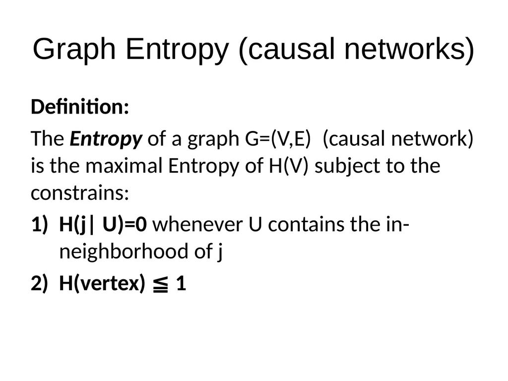
Graph Entropy (causal networks) Definition:
The Entropy of a graph G=(V,E) (causal network) is the maximal Entropy of H(V) subject to the constrains:
H(j| U)=0 whenever U contains the in-neighborhood of j
H(vertex) ≦ 1<br>
The Entropy of a graph G=(V,E) (causal network) is the maximal Entropy of H(V) subject to the constrains:
H(j| U)=0 whenever U contains the in-neighborhood of j
H(vertex) ≦ 1<br>
18
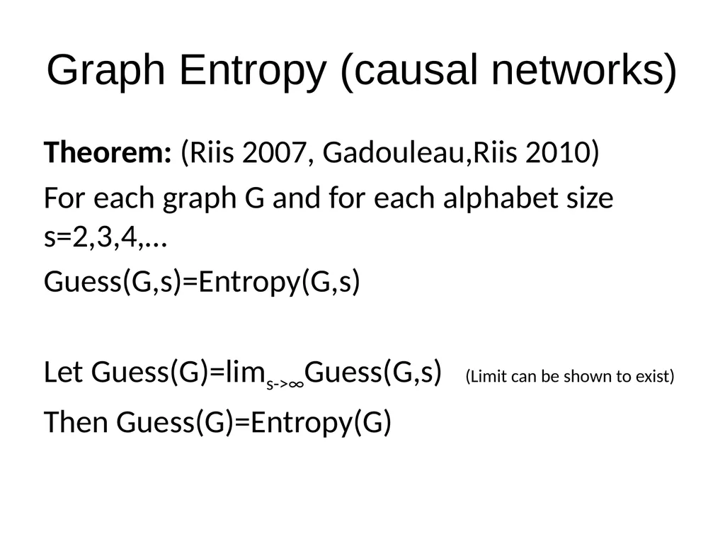
Graph Entropy (causal networks) Theorem: (Riis 2007, Gadouleau,Riis 2010)
For each graph G and for each alphabet size s=2,3,4,…
Guess(G,s)=Entropy(G,s)
Let Guess(G)=lims->∞Guess(G,s) (Limit can be shown to exist)
Then Guess(G)=Entropy(G)<br>
For each graph G and for each alphabet size s=2,3,4,…
Guess(G,s)=Entropy(G,s)
Let Guess(G)=lims->∞Guess(G,s) (Limit can be shown to exist)
Then Guess(G)=Entropy(G)<br>
19
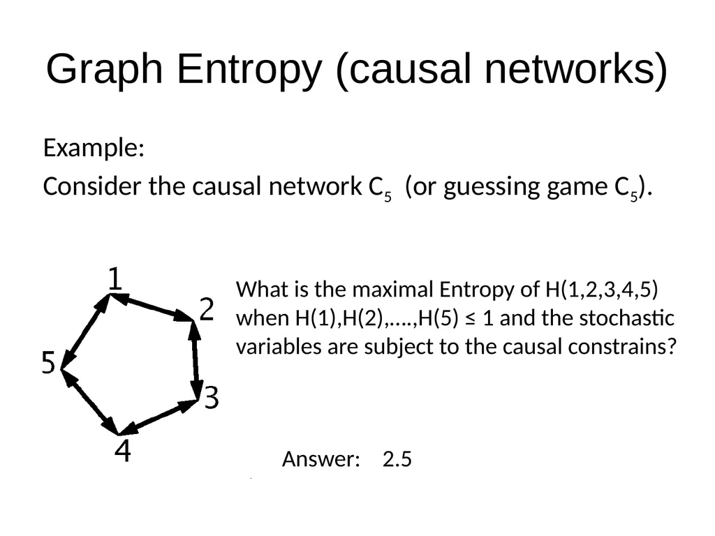
Graph Entropy (causal networks) Example:
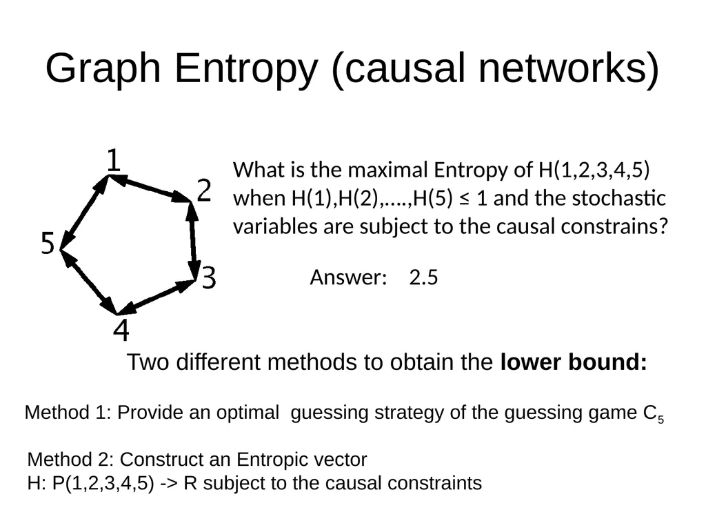
Consider the causal network C5 (or guessing game C5). What is the maximal Entropy of H(1,2,3,4,5)
when H(1),H(2),….,H(5) ≤ 1 and the stochastic
variables are subject to the causal constrains? Answer: 2.5<br>
Consider the causal network C5 (or guessing game C5). What is the maximal Entropy of H(1,2,3,4,5)
when H(1),H(2),….,H(5) ≤ 1 and the stochastic
variables are subject to the causal constrains? Answer: 2.5<br>
20
Graph Entropy (causal networks) What is the maximal Entropy of H(1,2,3,4,5)
when H(1),H(2),….,H(5) ≤ 1 and the stochastic
variables are subject to the causal constrains? Answer: 2.5 Two different methods to obtain the lower bound: Method 1: Provide an optimal guessing strategy of the guessing game C5 Method 2: Construct an Entropic vector
H: P(1,2,3,4,5) -> R subject to the causal constraints<br>
when H(1),H(2),….,H(5) ≤ 1 and the stochastic
variables are subject to the causal constrains? Answer: 2.5 Two different methods to obtain the lower bound: Method 1: Provide an optimal guessing strategy of the guessing game C5 Method 2: Construct an Entropic vector
H: P(1,2,3,4,5) -> R subject to the causal constraints<br>
21
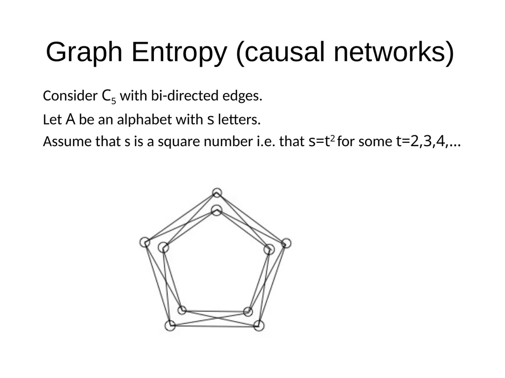
Graph Entropy (causal networks) Consider C5 with bi-directed edges.
Let A be an alphabet with s letters.
Assume that s is a square number i.e. that s=t2 for some t=2,3,4,…<br>
Let A be an alphabet with s letters.
Assume that s is a square number i.e. that s=t2 for some t=2,3,4,…<br>
22
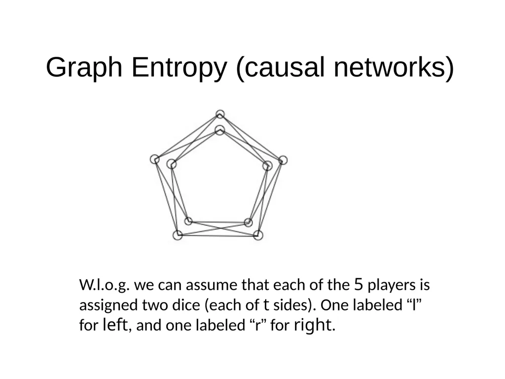
Graph Entropy (causal networks) W.l.o.g. we can assume that each of the 5 players is assigned two dice (each of t sides). One labeled “l” for left, and one labeled “r” for right.<br>
23
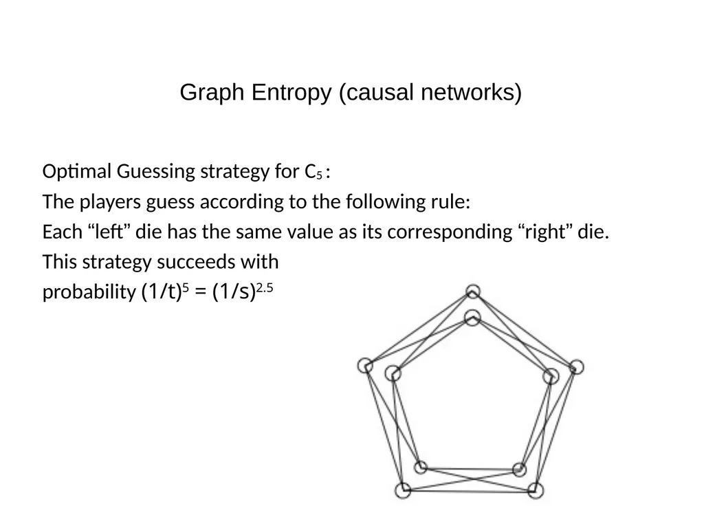
Graph Entropy (causal networks) Optimal Guessing strategy for C5 :
The players guess according to the following rule:
Each “left” die has the same value as its corresponding “right” die.
This strategy succeeds with
probability (1/t)5 = (1/s)2.5<br>
The players guess according to the following rule:
Each “left” die has the same value as its corresponding “right” die.
This strategy succeeds with
probability (1/t)5 = (1/s)2.5<br>
24
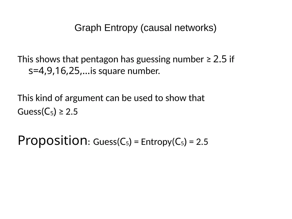
Graph Entropy (causal networks) This shows that pentagon has guessing number ≥ 2.5 if s=4,9,16,25,…is square number.
This kind of argument can be used to show that
Guess(C5) ≥ 2.5
Proposition: Guess(C5) = Entropy(C5) = 2.5<br>
This kind of argument can be used to show that
Guess(C5) ≥ 2.5
Proposition: Guess(C5) = Entropy(C5) = 2.5<br>
25
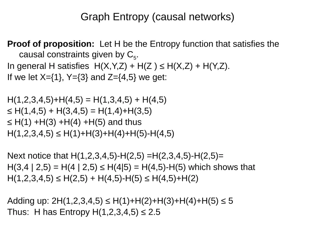
Graph Entropy (causal networks) Proof of proposition: Let H be the Entropy function that satisfies the causal constraints given by C5.
In general H satisfies H(X,Y,Z) + H(Z ) ≤ H(X,Z) + H(Y,Z).
If we let X={1}, Y={3} and Z={4,5} we get:
H(1,2,3,4,5)+H(4,5) = H(1,3,4,5) + H(4,5)
≤ H(1,4,5) + H(3,4,5) = H(1,4)+H(3,5)
≤ H(1) +H(3) +H(4) +H(5) and thus
H(1,2,3,4,5) ≤ H(1)+H(3)+H(4)+H(5)-H(4,5)
Next notice that H(1,2,3,4,5)-H(2,5) =H(2,3,4,5)-H(2,5)=
H(3,4 | 2,5) = H(4 | 2,5) ≤ H(4|5) = H(4,5)-H(5) which shows that
H(1,2,3,4,5) ≤ H(2,5) + H(4,5)-H(5) ≤ H(4,5)+H(2)
Adding up: 2H(1,2,3,4,5) ≤ H(1)+H(2)+H(3)+H(4)+H(5) ≤ 5
Thus: H has Entropy H(1,2,3,4,5) ≤ 2.5<br>
In general H satisfies H(X,Y,Z) + H(Z ) ≤ H(X,Z) + H(Y,Z).
If we let X={1}, Y={3} and Z={4,5} we get:
H(1,2,3,4,5)+H(4,5) = H(1,3,4,5) + H(4,5)
≤ H(1,4,5) + H(3,4,5) = H(1,4)+H(3,5)
≤ H(1) +H(3) +H(4) +H(5) and thus
H(1,2,3,4,5) ≤ H(1)+H(3)+H(4)+H(5)-H(4,5)
Next notice that H(1,2,3,4,5)-H(2,5) =H(2,3,4,5)-H(2,5)=
H(3,4 | 2,5) = H(4 | 2,5) ≤ H(4|5) = H(4,5)-H(5) which shows that
H(1,2,3,4,5) ≤ H(2,5) + H(4,5)-H(5) ≤ H(4,5)+H(2)
Adding up: 2H(1,2,3,4,5) ≤ H(1)+H(2)+H(3)+H(4)+H(5) ≤ 5
Thus: H has Entropy H(1,2,3,4,5) ≤ 2.5<br>
26
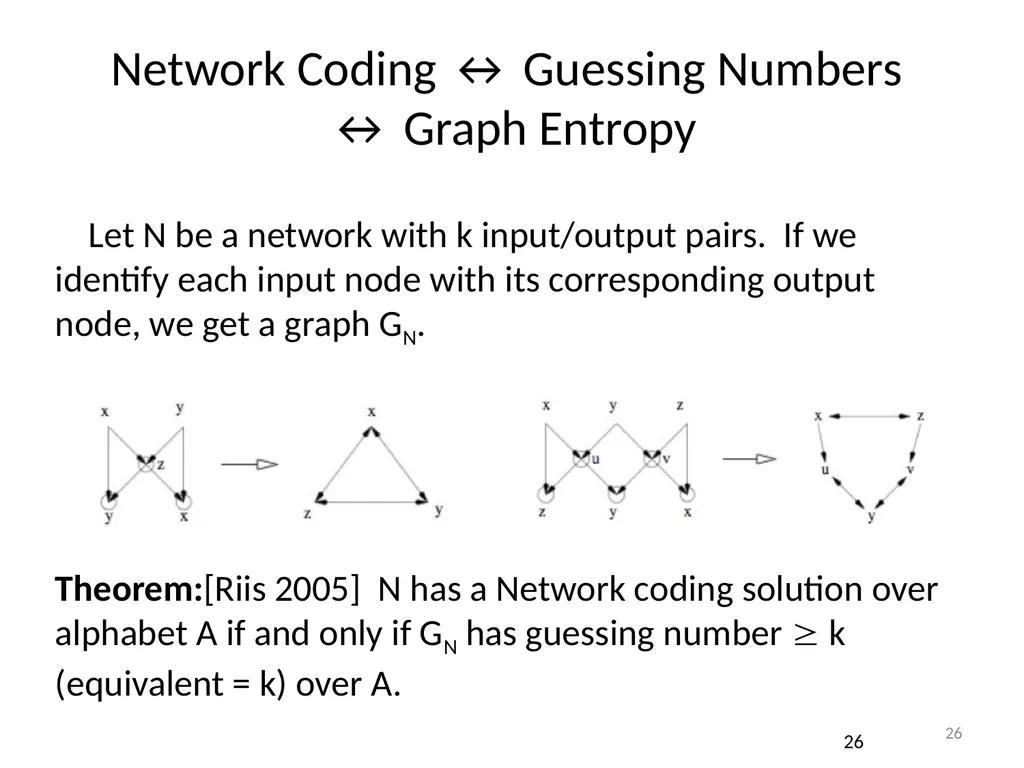
26 Network Coding ↔ Guessing Numbers
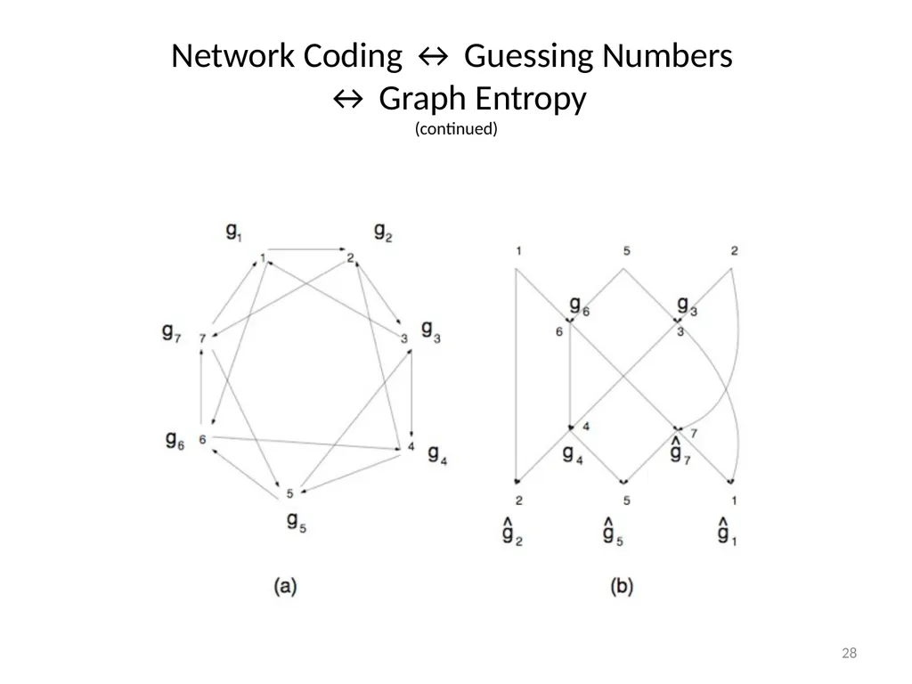
↔ Graph Entropy Let N be a network with k input/output pairs. If we identify each input node with its corresponding output node, we get a graph GN.
Theorem:[Riis 2005] N has a Network coding solution over alphabet A if and only if GN has guessing number ≥ k (equivalent = k) over A. 26<br>
Theorem:[Riis 2005] N has a Network coding solution over alphabet A if and only if GN has guessing number ≥ k (equivalent = k) over A. 26<br>
27
27 Network Coding ↔ Guessing Numbers
↔ Graph Entropy
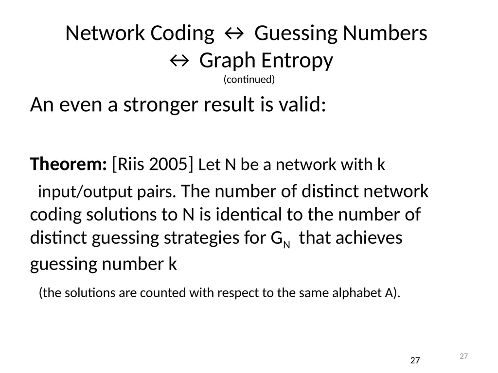
(continued) An even a stronger result is valid:
Theorem: [Riis 2005] Let N be a network with k
input/output pairs. The number of distinct network coding solutions to N is identical to the number of distinct guessing strategies for GN that achieves guessing number k
(the solutions are counted with respect to the same alphabet A). 27<br>
Theorem: [Riis 2005] Let N be a network with k
input/output pairs. The number of distinct network coding solutions to N is identical to the number of distinct guessing strategies for GN that achieves guessing number k
(the solutions are counted with respect to the same alphabet A). 27<br>
28
28 Network Coding ↔ Guessing Numbers
↔ Graph Entropy
(continued)<br>
29
29 Network Coding ↔ Guessing Numbers
↔ Graph Entropy
(continued)<br>
30
30 Network Coding ↔ Guessing Numbers
↔ Graph Entropy
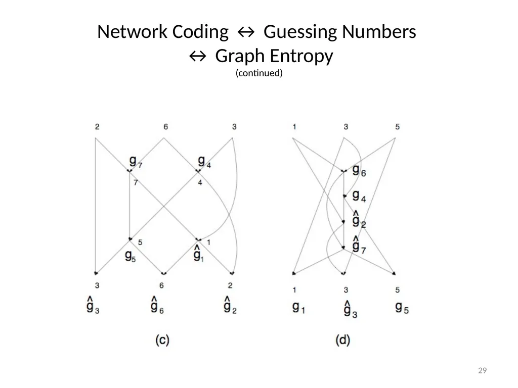
(continued) The networks in b, c and d all appear by “splitting” the graph G in a.
“Splitting” is the opposite operation as identifying
input/output pairs.
The networks in b, c and d have exactly the same number of network coding solutions (over a fixed alphabet A). This number is identical to the number of guessing strategies (over A) that achieve guessing number 3 for G. 30<br>
“Splitting” is the opposite operation as identifying
input/output pairs.
The networks in b, c and d have exactly the same number of network coding solutions (over a fixed alphabet A). This number is identical to the number of guessing strategies (over A) that achieve guessing number 3 for G. 30<br>
31
Examples and some basic results<br>
32
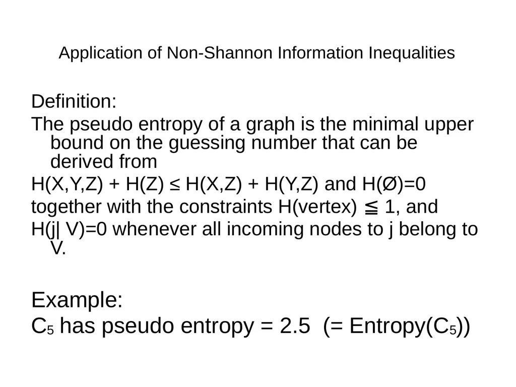
Application of Non-Shannon Information Inequalities Definition:
The pseudo entropy of a graph is the minimal upper bound on the guessing number that can be derived from
H(X,Y,Z) + H(Z) ≤ H(X,Z) + H(Y,Z) and H(Ø)=0
together with the constraints H(vertex) ≦ 1, and
H(j| V)=0 whenever all incoming nodes to j belong to V.
Example:
C5 has pseudo entropy = 2.5 (= Entropy(C5))<br>
The pseudo entropy of a graph is the minimal upper bound on the guessing number that can be derived from
H(X,Y,Z) + H(Z) ≤ H(X,Z) + H(Y,Z) and H(Ø)=0
together with the constraints H(vertex) ≦ 1, and
H(j| V)=0 whenever all incoming nodes to j belong to V.
Example:
C5 has pseudo entropy = 2.5 (= Entropy(C5))<br>
33
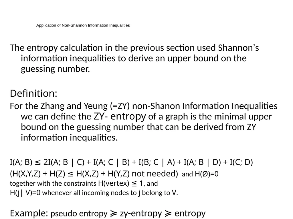
Application of Non-Shannon Information Inequalities The entropy calculation in the previous section used Shannon’s information inequalities to derive an upper bound on the guessing number.
Definition:
For the Zhang and Yeung (=ZY) non-Shanon Information Inequalities we can define the ZY- entropy of a graph is the minimal upper bound on the guessing number that can be derived from ZY information inequalities.
I(A; B) ≤ 2I(A; B | C) + I(A; C | B) + I(B; C | A) + I(A; B | D) + I(C; D)
(H(X,Y,Z) + H(Z) ≤ H(X,Z) + H(Y,Z) not needed) and H(Ø)=0
together with the constraints H(vertex) ≦ 1, and
H(j| V)=0 whenever all incoming nodes to j belong to V.
Example: pseudo entropy ≽ zy-entropy ≽ entropy<br>
Definition:
For the Zhang and Yeung (=ZY) non-Shanon Information Inequalities we can define the ZY- entropy of a graph is the minimal upper bound on the guessing number that can be derived from ZY information inequalities.
I(A; B) ≤ 2I(A; B | C) + I(A; C | B) + I(B; C | A) + I(A; B | D) + I(C; D)
(H(X,Y,Z) + H(Z) ≤ H(X,Z) + H(Y,Z) not needed) and H(Ø)=0
together with the constraints H(vertex) ≦ 1, and
H(j| V)=0 whenever all incoming nodes to j belong to V.
Example: pseudo entropy ≽ zy-entropy ≽ entropy<br>
34
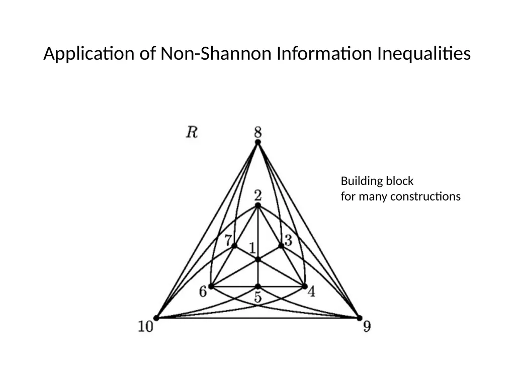
Application of Non-Shannon Information Inequalities Building block
for many constructions<br>
for many constructions<br>
35
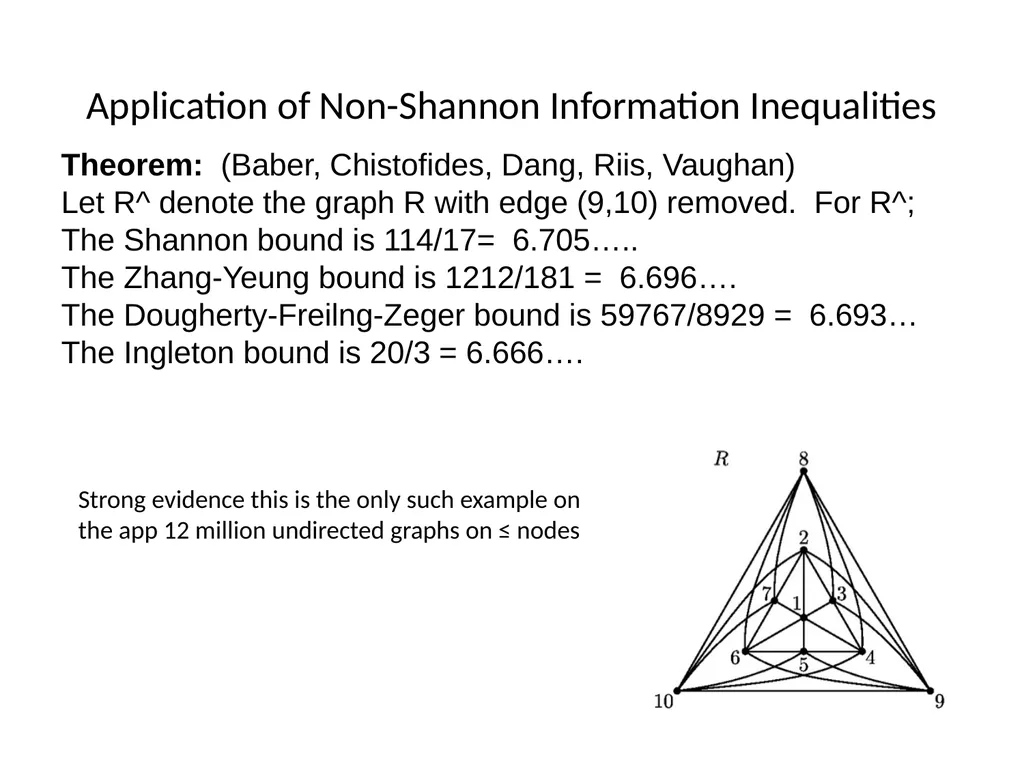
Application of Non-Shannon Information Inequalities Theorem: (Baber, Chistofides, Dang, Riis, Vaughan)
Let R^ denote the graph R with edge (9,10) removed. For R^;
The Shannon bound is 114/17= 6.705…..
The Zhang-Yeung bound is 1212/181 = 6.696….
The Dougherty-Freilng-Zeger bound is 59767/8929 = 6.693…
The Ingleton bound is 20/3 = 6.666…. Strong evidence this is the only such example on
the app 12 million undirected graphs on ≤ nodes<br>
Let R^ denote the graph R with edge (9,10) removed. For R^;
The Shannon bound is 114/17= 6.705…..
The Zhang-Yeung bound is 1212/181 = 6.696….
The Dougherty-Freilng-Zeger bound is 59767/8929 = 6.693…
The Ingleton bound is 20/3 = 6.666…. Strong evidence this is the only such example on
the app 12 million undirected graphs on ≤ nodes<br>
36
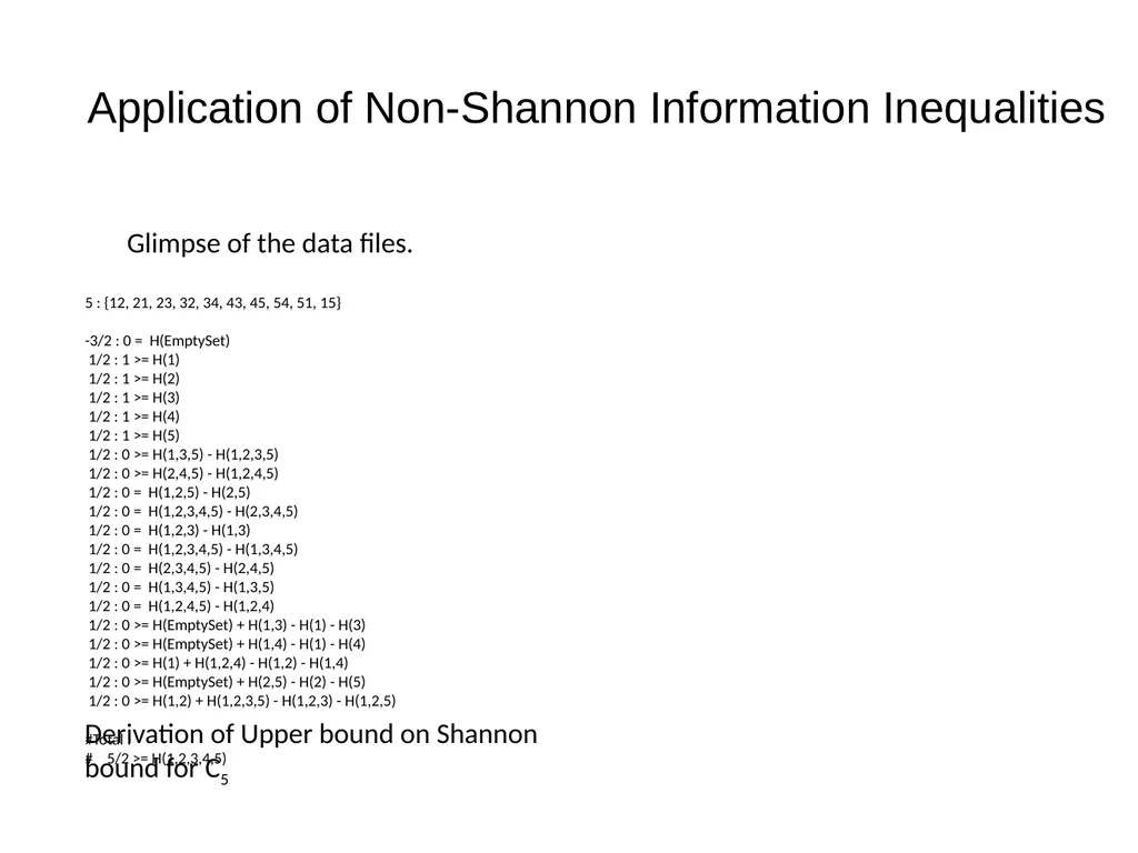
Application of Non-Shannon Information Inequalities 5 : {12, 21, 23, 32, 34, 43, 45, 54, 51, 15}
-3/2 : 0 = H(EmptySet)
1/2 : 1 >= H(1)
1/2 : 1 >= H(2)
1/2 : 1 >= H(3)
1/2 : 1 >= H(4)
1/2 : 1 >= H(5)
1/2 : 0 >= H(1,3,5) - H(1,2,3,5)
1/2 : 0 >= H(2,4,5) - H(1,2,4,5)
1/2 : 0 = H(1,2,5) - H(2,5)
1/2 : 0 = H(1,2,3,4,5) - H(2,3,4,5)
1/2 : 0 = H(1,2,3) - H(1,3)
1/2 : 0 = H(1,2,3,4,5) - H(1,3,4,5)
1/2 : 0 = H(2,3,4,5) - H(2,4,5)
1/2 : 0 = H(1,3,4,5) - H(1,3,5)
1/2 : 0 = H(1,2,4,5) - H(1,2,4)
1/2 : 0 >= H(EmptySet) + H(1,3) - H(1) - H(3)
1/2 : 0 >= H(EmptySet) + H(1,4) - H(1) - H(4)
1/2 : 0 >= H(1) + H(1,2,4) - H(1,2) - H(1,4)
1/2 : 0 >= H(EmptySet) + H(2,5) - H(2) - H(5)
1/2 : 0 >= H(1,2) + H(1,2,3,5) - H(1,2,3) - H(1,2,5)
#Total :
# 5/2 >= H(1,2,3,4,5) Glimpse of the data files. Derivation of Upper bound on Shannon
bound for C5<br>
bound for C5<br>
37
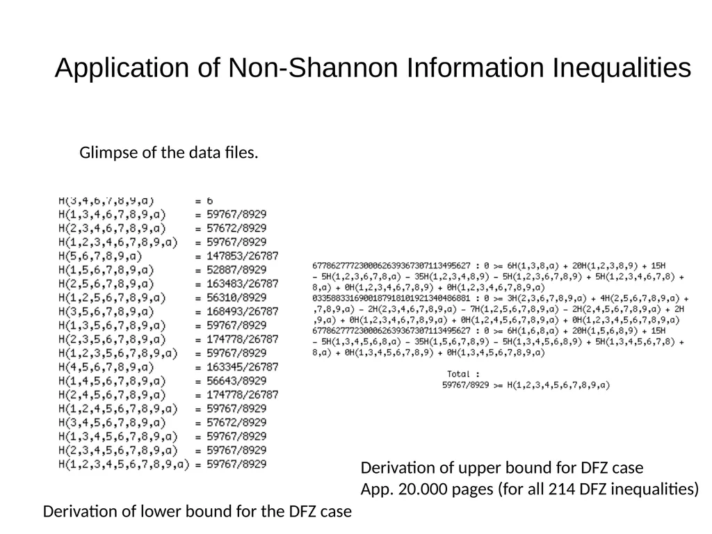
Application of Non-Shannon Information Inequalities Glimpse of the data files. Derivation of lower bound for the DFZ case Derivation of upper bound for DFZ case
App. 20.000 pages (for all 214 DFZ inequalities)<br>
App. 20.000 pages (for all 214 DFZ inequalities)<br>
38
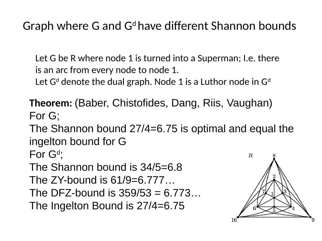
Graph where G and Gd have different Shannon bounds Let G be R where node 1 is turned into a Superman; I.e. there is an arc from every node to node 1.
Let Gd denote the dual graph. Node 1 is a Luthor node in Gd Theorem: (Baber, Chistofides, Dang, Riis, Vaughan)
For G;
The Shannon bound 27/4=6.75 is optimal and equal the
ingelton bound for G
For Gd;
The Shannon bound is 34/5=6.8
The ZY-bound is 61/9=6.777…
The DFZ-bound is 359/53 = 6.773…
The Ingelton Bound is 27/4=6.75<br>
Let Gd denote the dual graph. Node 1 is a Luthor node in Gd Theorem: (Baber, Chistofides, Dang, Riis, Vaughan)
For G;
The Shannon bound 27/4=6.75 is optimal and equal the
ingelton bound for G
For Gd;
The Shannon bound is 34/5=6.8
The ZY-bound is 61/9=6.777…
The DFZ-bound is 359/53 = 6.773…
The Ingelton Bound is 27/4=6.75<br>
39
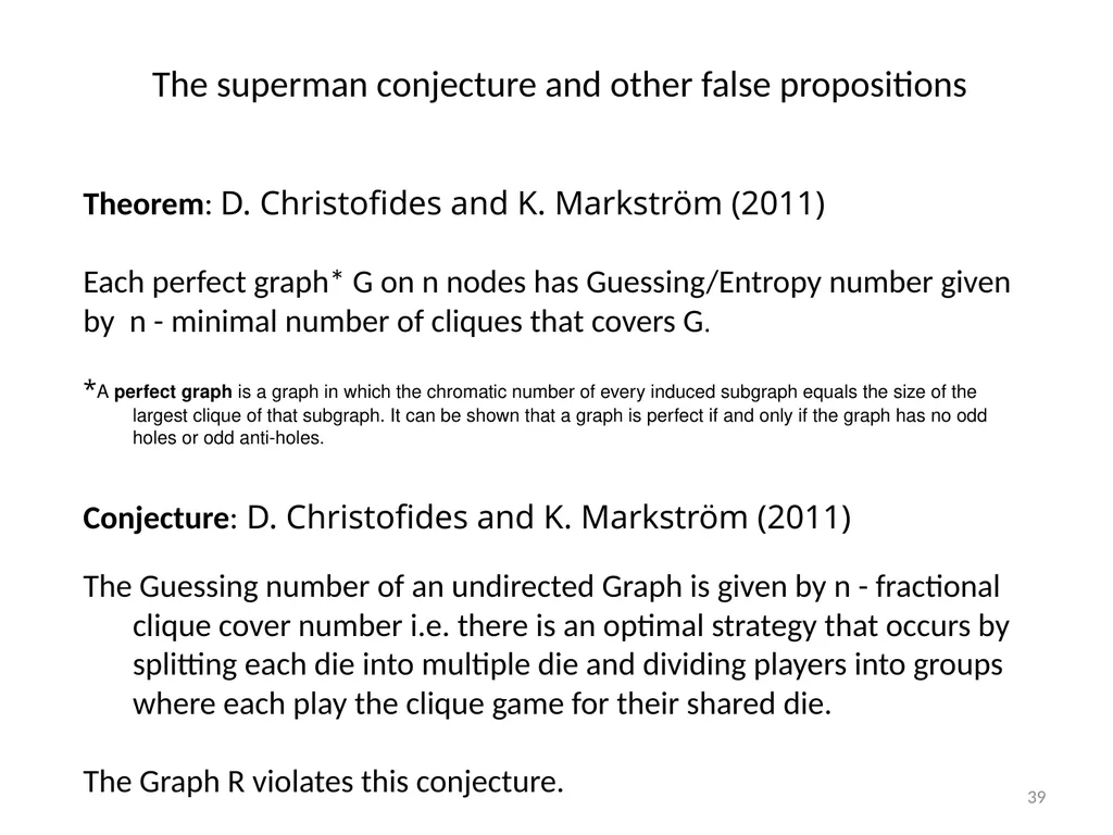
39 The superman conjecture and other false propositions Theorem: D. Christofides and K. Markström (2011)
Each perfect graph* G on n nodes has Guessing/Entropy number given
by n - minimal number of cliques that covers G.
*A perfect graph is a graph in which the chromatic number of every induced subgraph equals the size of the largest clique of that subgraph. It can be shown that a graph is perfect if and only if the graph has no odd holes or odd anti-holes.
Conjecture: D. Christofides and K. Markström (2011)
The Guessing number of an undirected Graph is given by n - fractional clique cover number i.e. there is an optimal strategy that occurs by splitting each die into multiple die and dividing players into groups where each play the clique game for their shared die.
The Graph R violates this conjecture.<br>
Each perfect graph* G on n nodes has Guessing/Entropy number given
by n - minimal number of cliques that covers G.
*A perfect graph is a graph in which the chromatic number of every induced subgraph equals the size of the largest clique of that subgraph. It can be shown that a graph is perfect if and only if the graph has no odd holes or odd anti-holes.
Conjecture: D. Christofides and K. Markström (2011)
The Guessing number of an undirected Graph is given by n - fractional clique cover number i.e. there is an optimal strategy that occurs by splitting each die into multiple die and dividing players into groups where each play the clique game for their shared die.
The Graph R violates this conjecture.<br>
40
The superman conjecture and other false propositions Superman conjecture/question: Does there exist an undirected graph whose asymptotic guessing number increases when a single directed edge is added?
We were able to clone a part of R to achieve a graph Rc on 13 nodes that provides a counter example to the superman conjecture.<br>
We were able to clone a part of R to achieve a graph Rc on 13 nodes that provides a counter example to the superman conjecture.<br>
41
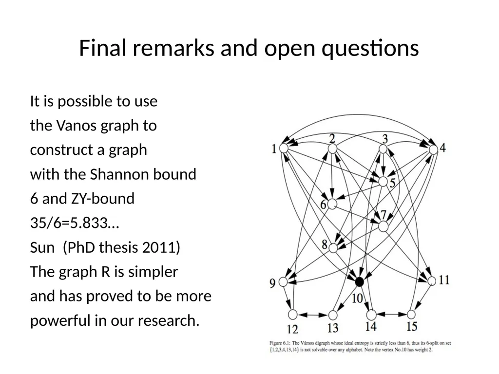
Final remarks and open questions It is possible to use
the Vanos graph to
construct a graph
with the Shannon bound
6 and ZY-bound
35/6=5.833…
Sun (PhD thesis 2011)
The graph R is simpler
and has proved to be more
powerful in our research.<br>
the Vanos graph to
construct a graph
with the Shannon bound
6 and ZY-bound
35/6=5.833…
Sun (PhD thesis 2011)
The graph R is simpler
and has proved to be more
powerful in our research.<br>
42
Final remarks and Open Questions Is it possible to amplify the above result and construct graph(s) where there is a substantial gap between the pseudo Entropy, the zy-Entropy and the genuine Entropy?
Improve the upper bounds and the lower bounds for the Entropy of R^
Can generalize the causal structures (Graphs) to lattices.
Do the graphs G and Gd have different graph entropies?<br>
Improve the upper bounds and the lower bounds for the Entropy of R^
Can generalize the causal structures (Graphs) to lattices.
Do the graphs G and Gd have different graph entropies?<br>
43
43 Final Remarks and Open Problems Spin off: Network Coding, Guessing Game and Graph entropy approach have lead to new areas of research
Combinatorial Representations (2011) (With Peter Cameron and Max Gadouleau)
A generalisation of Matroid theory
Memoryless computation (2011) (With Max Gadouleau)
Dynamic communication networks (2011) (With Max Gadouleau)
Graph entropy and non-Shannon information inequalities (Yun Sun PhD Thesis 2011)
Construction of new classes of communication networks (with Max Gadouleau) (2010)
New max-flow min-cut theorem for multiuser communication (with Max Gadouleau) (2011)
Thank you 33<br>
Combinatorial Representations (2011) (With Peter Cameron and Max Gadouleau)
A generalisation of Matroid theory
Memoryless computation (2011) (With Max Gadouleau)
Dynamic communication networks (2011) (With Max Gadouleau)
Graph entropy and non-Shannon information inequalities (Yun Sun PhD Thesis 2011)
Construction of new classes of communication networks (with Max Gadouleau) (2010)
New max-flow min-cut theorem for multiuser communication (with Max Gadouleau) (2011)
Thank you 33<br>